Example: Basis pursuit denoising (BPD)

In this example, a noisy speech waveform is denoised using basis pursuit denoising (BPD) and an oversampled DFT.

Ivan Selesnick
NYU-Poly
selesi@poly.edu
March 2012

Start
Load signal
Make noisy signal
Spectrum of noisy signal
Basis pursuit denoising
Compute denoised signal

Start

close all
clear
MyGraphPrefsON

printme = @(txt) print('-deps', sprintf('figures/Example_BPD_%s',txt));

randn('state',0);       % set state so as to exactly reproduce example

Load signal

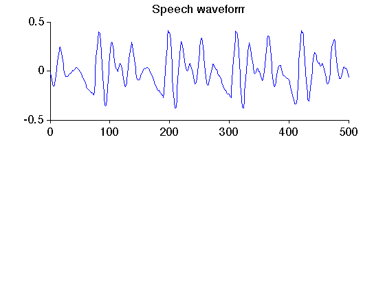
Load speech waveform data

[sp1, fs] = wavread('data/sp1.wav');

M = 500;                        % M : length of signal
s = sp1(5500+(1:M));            % s : signal (without noise)

figure(1)
clf
subplot(2,1,1)
plot(s)
box off
title('Speech waveform')

fprintf('Sampling rate: %d samples/second \n', fs)

Sampling rate: 16000 samples/second

Make noisy signal

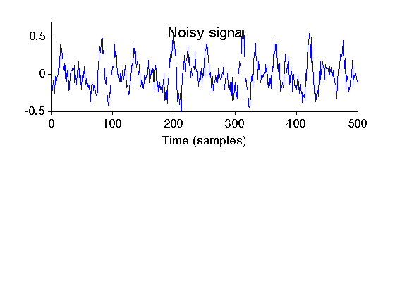
Make noisy signal by adding white Gaussian noise

w = 0.1 * randn(M,1);      % w : zero-mean Gaussian noise
y = s + w;                 % y : noisy speech signal

figure(2)
clf
subplot(2,1,1)
plot(y)
box off
ylim1 = [-0.5 0.7];
ylim(ylim1);
mytitle('Noisy signal');
xlabel('Time (samples)')
printme('noisy')

Spectrum of noisy signal

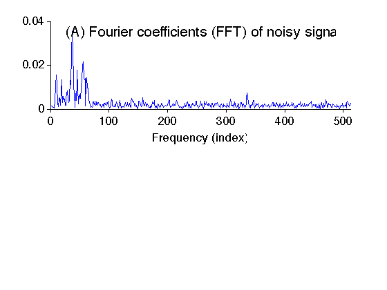
Compute the spectrum of the noisy signal 'y' using the oversampled DFT.

N = 2^10;                   % N : Length of Fourier coefficient vector

Y = (1/N)*fft(y,N);         % Y : Spectrum of noisy signal

figure(1)
clf
subplot(2,1,1)
plot(abs(Y))
xlim([0 N/2])
box off
mytitle('(A) Fourier coefficients (FFT) of noisy signal');
xlabel('Frequency (index)')
printme('noisy_spectrum')

Basis pursuit denoising

Perform basis pursuit denoising using iteratitive algorithm.

% Define functions (Matlab function handles)
H = @(x) A(x,M,N);          % H : converts coefficients to signal
HT = @(x) AT(x,M,N);        % HT : converts signal to coefficients
p = N;                      % p : Parseval constant H*HT = p*Identity

% Define algorithm parameters
lambda = 7;                 % lambda : regularization parameter
Nit = 50;                   % Nit : number of iterations
mu = 500;                   % mu : ADMM parameter

% Run BPD algorithm
[c, cost] = bpd_salsa(y, H, HT, p, lambda, mu, Nit);

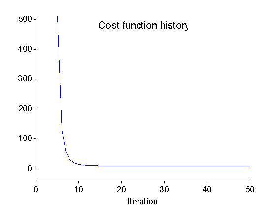
Display cost function history of BPD algorithm

figure(1)
clf
plot(cost)
mytitle('Cost function history');
xlabel('Iteration')
it1 = 5;
del = cost(it1) - min(cost);
ylim([min(cost)-0.1*del cost(it1)])
xlim([0 Nit])
box off
printme('CostFunction')

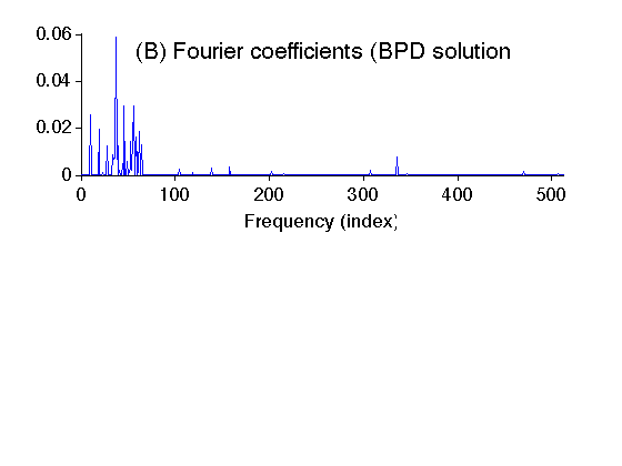
Display BPD Fourier coefficients

figure(1)
clf
subplot(2,1,1)
plot(abs(c))
xlim([0 N/2])
box off
mytitle('(B) Fourier coefficients (BPD solution)');
xlabel('Frequency (index)')
printme('bpd_spectrum')

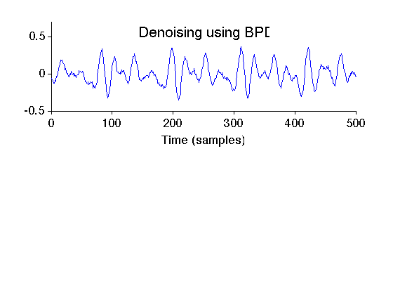
Compute denoised signal

g = H(c);
g = real(g);

figure(1)
clf
subplot(2,1,1)
plot(g)
box off
ylim(ylim1);
mytitle('Denoising using BPD');
xlabel('Time (samples)')
printme('BPD')

MyGraphPrefsOFF