demo_filter_matrices
Illustration of low-pass and high-pass linear filters uing banded filter matrices.
Ivan Selesnick,
selesi@nyu.edu,
Tandon School of Engineering
New York University
2017
Contents
Start
clear

printme = @(filename) print('-dpdf', sprintf('figures/demo_filter_matrices_%s', filename));
Define high-pass filter H
N = 100;       % N : signal length
fc = 0.05;     % fc : cut-off frequency (cycles/sample) (0 < fc < 0.5)
d = 2;         % d : degree of filter is 2d (d = 1, 2, 3)

[A, B, B1, D, a, b] = ABfilt(d, fc, N);
H = @(x) A\(B*x);            % H : high-pass filter
L = @(x) x - H(x);           % L : low-pass filter
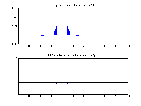
Impulse responses of filters
no = 40;
x = zeros(N,1); x(no) = 1;     % input signal (impulse)

figure(1)
clf
subplot(2, 1, 1)
stem(1:N, L(x), '.')
title(sprintf('LPF impulse response (impulse at n = %d)', no))

subplot(2, 1, 2)
stem(1:N, H(x), '.')
title(sprintf('HPF impulse response (impulse at n = %d)', no))
printme('impulse_responses')
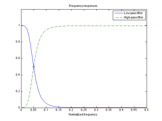
Frequency response of filters
% difference equation coefficients of low-pass filter
b_lpf = a - b;
a_lpf = a;

% Compute frequency response
[Hf_hpf, om] = freqz(b, a);
[Hf_lpf, om] = freqz(b_lpf, a_lpf);

figure(1)
clf
plot(om/pi/2, abs(Hf_lpf), om/pi/2, abs(Hf_hpf), '--')
line(fc, 0.5, 'marker', 'o')
title('Frequency responses')
legend('Low-pass filter', 'High-pass filter')
xlabel('Normalized frequency')
ylim([0 1.2])
printme('frequency_responses')
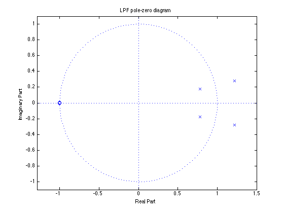
Pole-zero diagram of low-pass filter L
figure(1)
clf
[hz, hp, hl] = zplane(b_lpf, a_lpf);
title('LPF pole-zero diagram')
printme('zplane_LPF')
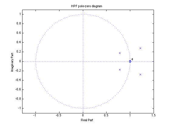
Pole-zero diagram of high-pass filter H
figure(1)
clf
zplane(b, a);
title('HPF pole-zero diagram')
printme('zplane_HPF')
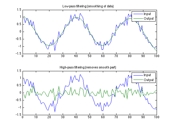
Filter noisy data
% Create noisy data
n = (1:N)';
x = cos(0.05*pi*n) + 0.2*randn(N,1);    % x : noisy data

y_lpf = L(x);               % Apply LPF to noisy data
y_hpf = H(x);               % Apply HPF to noisy data

figure(1)
clf
subplot(2, 1, 1)
plot(n, x, '.-', n, y_lpf, '-')
legend('Input', 'Output')
title('Low-pass filtering (smoothing of data)')

subplot(2, 1, 2)
plot(n, x, '.-', n, y_hpf, '-')
legend('Input', 'Output')
title('High-pass filtering (removes smooth part)')

printme('filtering')