demo_basic

Ivan Selesnick
NYU Tandon School of Engineering
2012, Revised 2016

Contents

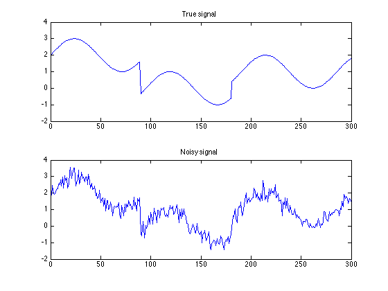
Create test data

clear

N = 300;        % N : length of signal
n = (1:N)';

s = load('data/basic_signal.txt');          % Load simulated ECG
y = load('data/basic_signal_noisy.txt');    % Load simulated noisy ECG

Plots

ax = [0 N -2 4];                        % ax : axis for plots

figure(1)
clf
subplot(2, 1, 1)
plot(s)
axis(ax)
title('True signal');

subplot(2, 1, 2)
plot(y)
axis(ax)
title('Noisy signal');

print -dpdf figures/demo_basic_data

Define low-pass filter

d = 2;          % d : filter order parameter (d = 1, 2, or 3)
fc = 0.022;     % fc : cut-off frequency (cycles/sample) (0 < fc < 0.5);

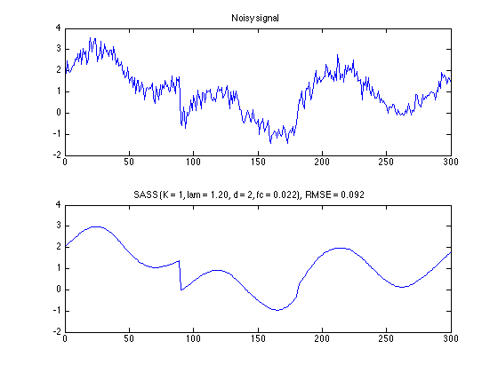
SASS - run algorithm

K = 1;          % K : order of sparse derivative
lam = 1.2;      % lam : regularization parameter

[x, u] = sass_L1(y, d, fc, K, lam);

err = s - x;
RMSE = sqrt(mean(err.^2));

0 incorrectly locked zeros detected.

SASS - plot denoised signal

txt = sprintf('SASS (K = %d, lam = %.2f, d = %d, fc = %.3f),  RMSE = %.3f', K, lam, d, fc, RMSE);

figure(1)
clf
subplot(2, 1, 1)
plot(n, y)
title('Noisy signal');
axis(ax)

subplot(2, 1, 2)
plot(n, x)
title(txt)
axis(ax)

print -dpdf figures/demo_basic_SASS

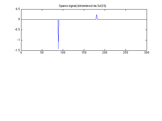
SASS - sparse signal component

figure(1)
clf
subplot(2, 1, 1)
plot(u)
title('Sparse signal (determined via SASS)')
xlim([0 N])

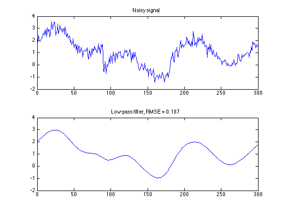
Compare to low-pass filter

[A, B] = ABfilt(d, fc, N, K);   % Filter matrices (banded)
H = @(x) A\(B*x);               % H : high-pass filter
L = @(x) x - H(x);              % L : low-pass filter

x_lpf = L(y);      % Low-pass filtering applied to noisy data

err = s - x_lpf;
RMSE_lpf = sqrt(mean(err.^2));

txt_lpf = sprintf('Low-pass filter, RMSE = %.3f', RMSE_lpf);

figure(1)
clf
subplot(2, 1, 1)
plot(n, y)
title('Noisy signal');
axis(ax)

subplot(2, 1, 2)
plot(n, x_lpf)
title(txt_lpf)
axis(ax)

print -dpdf figures/demo_basic_lowpass_filter

Published with MATLAB® 7.12