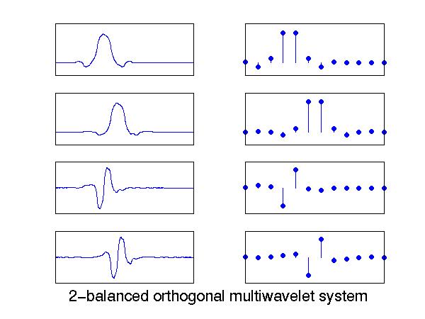
Even-length, 2-balanced

There are 8 different minimal-length pairs of scaling filters. The best solution, obtained using Gröbner bases, is shown in this figure, and is given by the formulas in the MATLAB program symbal2e.m. The numerical solutions are tabulated in the file symbal2e.float.

The scaling filters h0 and h1 were found by converting the nonlinear design equations (eqs) into a lexical Gröbner basis (gb.lp), and factorizing that into four disjoint Gröbner bases (gb.lp.fact.1, gb.lp.fact.2, gb.lp.fact.3, gb.lp.fact.4). All 8 minimal-length pairs of scaling filters can be found by solving these 4 Gröbner bases. Only 2 of the 8 solutions yield smooth scaling functions. The smoothest solution, shown in the figure, is given by one of the solutions of gb.lp.fact.2.

To obtain the wavelet filters h2 and h3, the nonlinear design equations (eqs.B) for the total system (scaling and wavelet filters) were appended to the Gröbner basis corresponding to the best scaling functions (gb.lp.fact.2). For this set of equations, the lexical Gröbner basis (gb.B.lp) was obtained, which yields both the scaling filters h0, h1 and the wavelet filters h2, h3 tabulated in the MATLAB program symbal2e.m. Note that in the design equations, the filters h0 and h1 are normalized so that the their DC gain is 1.

We also provide for this example the programs for reproducing the scaling filters: the Maple program for automatically generating the equations (setup) and the Singular program for obtaining the Gröbner bases (sfile). Executing these programs in sequence will regenerate the Gröbner bases gb.lp.fact.*. To generate the wavelet filters, we provide the Maple program for automatically generating the equations (setup.B), the Singular program for obtaining the Gröbner basis (sfile.B), and the Maple program for solving the the Gröbner basis (result.B). Executing these programs in sequence will regenerate the MATLAB program symbal2e.m.

Go back up.