Odd-length, 1-balanced
There are 4 different minimal-length pairs of scaling filters h0, h1 that satisfy the nonlinear design equations (eqs). They are tabulated in the MATLAB programs coeff1.m and coeff2.m. To obtain the 4 solutions, use the programs with the following syntax:
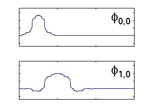
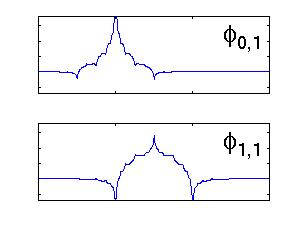
 [h0,h1] = coeff1(0)
 [h0,h1] = coeff1(1)
 [h0,h1] = coeff2(0)
 [h0,h1] = coeff2(1)
The only solution for which the scaling functions are continuous, [h0,h1] = coeff1(0), is shown in this figure.
Although for this example the design equations are simple enough to solve without them, Gröbner basis techniques provide a systematic approach. The lexical Gröbner basis (gb.lp), factorizes into two disjoint Gröbner bases (gb.lp.fact.1, gb.lp.fact.2). The scaling filters are obtained by solving these 2 Gröbner bases. Only 1 of the 4 solutions yields continuous scaling functions.
We also provide for this example the programs for reproducing the scaling filters: the Maple program for automatically generating the equations (setup), the Singular program for obtaining the Gröbner bases (sfile), and the Maple programs for solving the the Gröbner bases (result.1, result.2). Executing these programs in sequence will regenerate the coefficients.
Go back up.