LPFTVD_Example_1

This example illustrates the LPF/TVD algorithm: simultaneous low-pass filtering (LPF) and total variation denoising (TVD). The algorithm is based on majorization-minimization and fast solvers for banded linear systems.

Ivan Selesnick
Polytechnic Institute of NYU
2012

Contents

Start

clear
% close all

printme = @(filename) print('-dpdf', sprintf('figures/LPFTVD_Example_1_%s', filename));

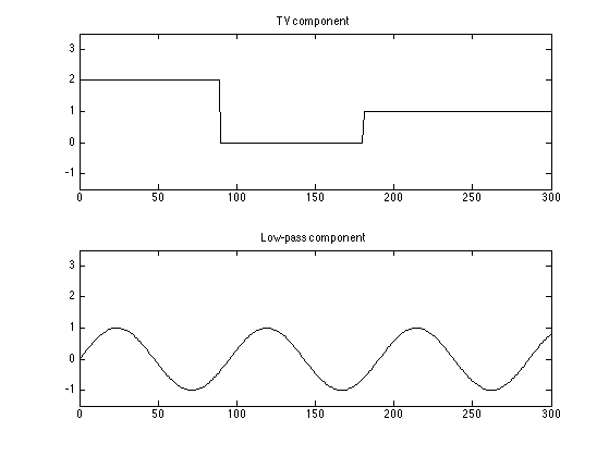
Create test signal

N = 300;                                    % N : length of signal
n = (1:N)';

s1 = 2*(n < 0.3*N) + 1*(n > 0.6*N);         % s1 : step function
s2 = sin(0.021*pi*n);                       % s2 : smooth function
s = s1 + s2;                                % s : total signal

ax = [0 N -1.5 3.5];                        % ax : axis for plots

figure(1)
clf

subplot(2, 1, 1)
plot(s1)
axis(ax)
title('TV component')

subplot(2, 1, 2)
plot(s2)
axis(ax)
title('Low-pass component')

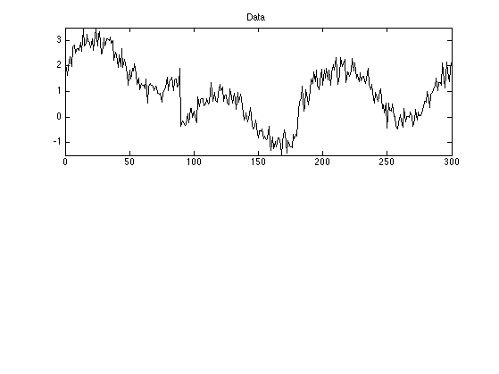
Create noisy signal

sigma = 0.3;                            % sigma : standard deviation of noise

randn('state', 0);                     % Set state so example is reproducible
noise = sigma*randn(N, 1);             % noise : white zero-mean Gaussian

y = s + noise;                          % y : noisy data

figure(1)
clf

subplot(2, 1, 1)
plot(y)
axis(ax)
title('Data');
printme('data')

Define high-pass filter H

The high-pass filter is H = A\B where A and B are banded matrices (sparse data type in MATLAB).

% Set filter parameters (fc, d)

d = 2;           % d : filter order parameter (d = 1, 2, or 3)

fc = 0.022;       % fc : cut-off frequency (cycles/sample) (0 < fc < 0.5);

[A, B, B1] = ABfilt(d, fc, N);

LPF/TVD algorithm

Run the LPF/TVD algorithm to perform simultaneous low-pass filtering (LPF) and total-variation denoising (TVD).

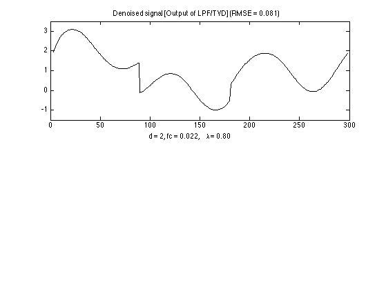
lam = 0.8;                              % lam : regularization parameter

Nit = 30;                               % Nit : number of iterations

[x, f, cost] = lpftvd(y, d, fc, lam, Nit);          % Run LPF/TVD algorithm
% x : TVD component
% f : LPF component

txt_params = sprintf('d = %d, fc = %.3f, \\lambda = %.2f', d, fc, lam);

err = s - x - f;
err = err(d+1:N-d);   % truncate NaNs.
rmse = sqrt(mean(err.^2));

fprintf('LPF/TVD (RMSE = %.3f)\n', rmse);


% txt = sprintf('LPF/TVD (RMSE = %.3f)', rmse);
% disp(txt)

LPF/TVD (RMSE = 0.081)

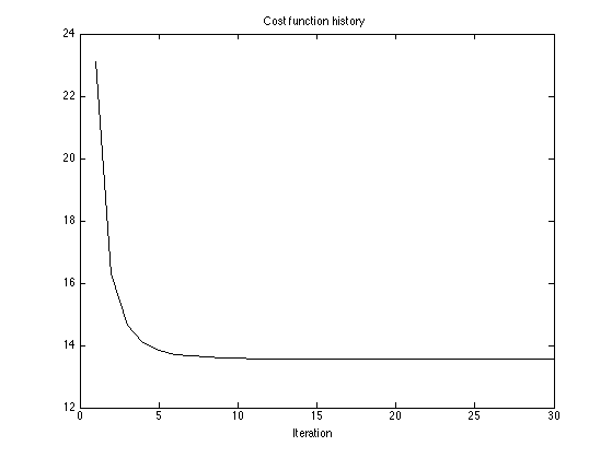
Cost function history

Show the cost function history to verify the convergence of the algorithm.

figure(1)
clf
plot(cost)
title('Cost function history');
xlabel('Iteration')

printme('cost')

Display output of LPF/TVD algorithm

Set mean of x to zero for convenience of plotting

mx = mean(x);
x = x - mx;
f = f + mx;

Display LPF/TVD output

figure(2)
clf

subplot(2, 1, 1)
plot(x + f)
axis(ax)
str = sprintf('Denoised signal [Output of LPF/TVD] (RMSE = %.3f)', rmse);
title(str)
xlabel(txt_params)
printme('lpftvd')

Display the two components separately (low-pass and sparse derivative)

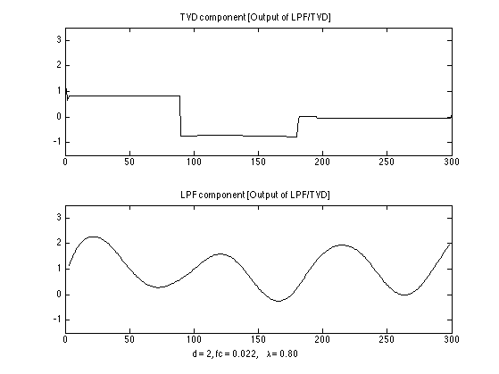
figure(2)
clf

subplot(2, 1, 1)
plot(x)
axis(ax)
title('TVD component [Output of LPF/TVD]');

subplot(2, 1, 2)
plot(f)
axis(ax)
title('LPF component [Output of LPF/TVD]');
xlabel(txt_params)

printme('lpftvd_components')

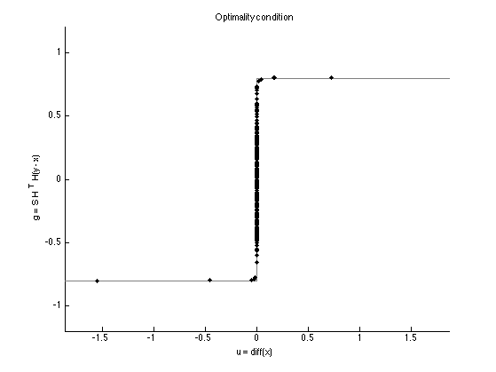
Verify optimality condition

Verify that the result obtained from lpftvd function satisfies the optimality conditions. (The scatter points should lie on the 'sign' function.)

AAT = A*A';
g = B1'*(AAT\(B*(y - x)));                      % same as S'H'H(y - x)

m = max(abs(diff(x)));

figure(1)
clf
line([-m 0 0 m]*1.2, [-1 -1 1 1]*lam, 'color', 0.5*[1 1 1])   % sign function
line(diff(x), g, 'marker', '.', 'linestyle', 'none', 'markersize', 10);  % scatter points
xlim([-1 1]*1.2*m)
ylim([-1 1]*1.5*lam)
ylabel('g = S H^T H(y - x)')
xlabel('u = diff(x)')
title('Optimality condition')

printme('optimality')

Published with MATLAB® 7.12