LPFCSD_Example_2

This example illustrates the LPF/CSD algorithm: simultaneous low-pass filtering (LPF) and compound sparsity denoising (CSD). The LPF/CSD algorithm is used to filter near infrared spectroscopic (NIRS) time series data.

The main parameters are:

d : Low-pass filter order = 2d
fc : Low-pass filter cut-off frequency (in cycles/sample)
lam0, lam1 : regularization parameters

Ivan Selesnick,
Polytechnic Institute of NYU,
June 2012

Start
Load data
Run LPF/CSD algorithm
Display output of LPF/CSD
Compare with band-pass filter (BPF)

Start

clear
close all

printme = @(filename) print('-dpdf', sprintf('figures/LPFCSD_Example_2_%s', filename));

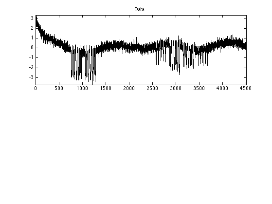
Load data

y = load('NIRS_data.txt');
y = y(:);
y = y - mean(y);
y = y * 1e4;

N = length(y);
n = 1:N;

figure(1)
clf

subplot(2,1,1)
plot(y);
xlim([0 N])
ylim1 = [min(y) max(y)];
ylim(ylim1)
title('Data');
printme('data')

Run LPF/CSD algorithm

Run LPF/CSD algorithm to perform simultaneous low-pass filtering and compound sparsity denoising.

% Set filter parameters
fc = 0.002;          % fc : cut-off frequency (cycles/sample)
d = 1;               % d : filter order parameter (d = 1, 2, or 3)

% lam0, lam1 : positive regularization parameters
lam0 = 0.05;
lam1 = 1;

% lam0 : increasing lam0 attenuates the signal x
% lam1 : increasing lam1 makes the signal x more flat (attenuates the first-order difference of x)
% Decreasing both lam0 and lam1 toward zero makes the algorithm behave like a low-pass filter.

Nit = 100;
% Nit : number of iterations (choose N large enough so that algorithm converges)

mu = 0.4;
% mu : ADMM parameter
% mu affects the convergence of the algorithm, but not the solution to
% which it converges.

[x, f, cost] = lpfcsd(y, d, fc, lam0, lam1, Nit, mu);       % Run LPF/CSD algorithm

txt = sprintf('fc = %.2e, lam0 = %.2e, lam1 = %.2e', fc, lam0, lam1);

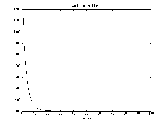
Display cost function history

figure(1)
clf
plot(cost)
title('Cost function history')
xlabel('Iteration')

% The cost function flattens out, indicating that the algorithm has converged.

Display output of LPF/CSD

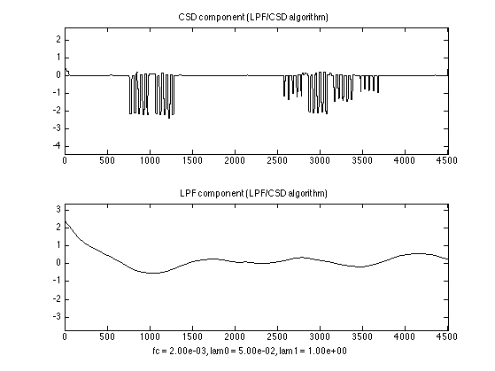
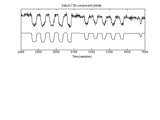
The LPF/CSD algorithm produces two output signals, denoted x and f. The output signal, x, is sparse and has a sparse deriviative. Observe that the signal x consists of the brief pulses present in the noisy data. The output signal, f, is a low-pass signal. Observe that the signal f closely follows the slowly-varying background trend present in the noisy data.

figure(2)
clf

subplot(2,1,1)
plot(x);
xlim([0 N])
title('CSD component (LPF/CSD algorithm)');
ylim(ylim1+(max(x)+min(x))/2-mean(ylim1))

subplot(2,1,2)
plot(f);
xlim([0 N])
title('LPF component (LPF/CSD algorithm)');
ylim(ylim1)
xlabel(txt)

printme('components')

Display detail

figure(1)
clf

subplot(2,1,1)
plot(n, y-mean(y) + 4, n, x)
xlim([0 N])
xlim([2800  3500])
set(gca, 'ytick', [])
title('Data & CSD component (detail)')
xlabel('Time (samples)')

printme('detail')

Compare with band-pass filter (BPF)

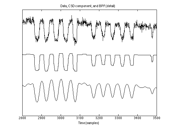
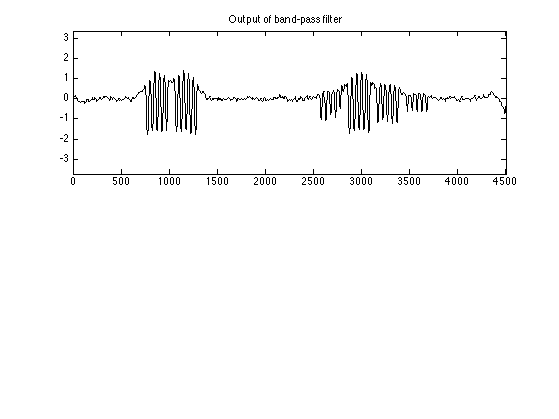
A band-pass filter is commonly used to isolate the brief pulses from the slowly varying background trend and to reduce the noise. However, observe that a band-pass filter distorts the shape of the brief pulses and exhibits a base-line drift coincident with the pulses. The LPF/CSD algorithm provides an alternative to the band-pass filter that reduces distortion and base-line drift issues.

[b2, a2] = butter(2, 0.08);                         % low-pass filter
[b3, a3] = butter(2, 0.005, 'high');                % high-pass filter

x_bpf = filtfilt(b3, a3, filtfilt(b2, a2, y) );     % perform band-pass filtering

figure(2)
clf

subplot(2,1,1)
plot(x_bpf);
xlim([0 N])
title('Output of band-pass filter');
ylim(ylim1)

printme('BPF')

Comparison detail