Example: Sparse deconvolution
Deconvolution of a spike signal with a comparison of two penalty functions. The algorithm is based on quadratic MM and uses a fast solver for banded systems.
Reference: Penalty and Shrinkage Functions for Sparse Signal Processing
Ivan Selesnick, NYU-Poly, selesi@poly.edu, 2012
http://eeweb.poly.edu/iselesni/lecture_notes/
Contents
Start
close all
clear
randn('state',0);           % set state so that example can be reproduced

printme = @(txt) print('-dpdf', sprintf('figures/Example_%s',txt));
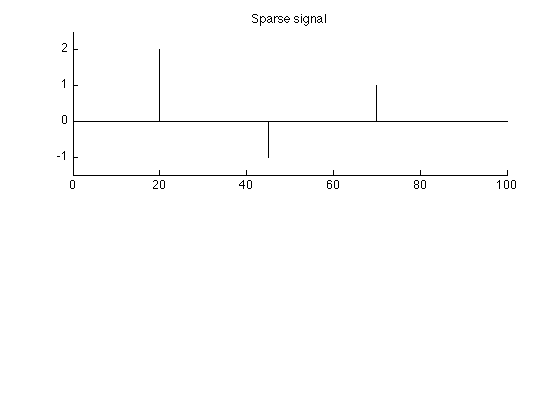
Create spike signal
N = 100;                    % N : length of signal
s = zeros(N,1);
k = [20 45 70];
a = [2 -1 1];               % a : spike amplitudes
s(k) = a;                   % s : spike signal

figure(1)
clf
subplot(2,1,1)
stem(s, 'marker', 'none')
box off
title('Sparse signal');
ylim1 = [-1.5 2.5];
ylim(ylim1)
printme('original')
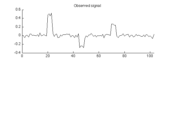
Create observed signal
The simulated observed signal is obtained by convolving the signal with a 4-point impulse response and adding noise.
L = 4;                      % L : length of impulse response
h = ones(L,1)/L;            % h : impulse response

M = N + L - 1;              % M : length of observed signal
sigma = 0.03;               % sigma : standard deviation of AWGN
w = sigma * randn(M,1);     % w : additive zero-mean Gaussian noise (AWGN)
y = conv(h,s) + w;          % y : observed data

figure(2)
clf
subplot(2,1,1)
plot(y)
box off
xlim([0 M])
title('Observed signal');
printme('observed')
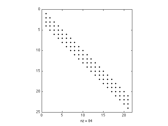
Create convolution matrix H
Create the convolution matrix H using Matlab sparse matrix functions 'sparse' and 'spdiags'. By making H a sparse matrix: - less memory is used, - multiplying vectors by H is faster, - fast algorithms for solving banded systems will be used.
H = sparse(M,N);
e = ones(N,1);
for i = 0:L-1
    H = H + spdiags(h(i+1)*e, -i, M, N);            % H : convolution matrix (sparse)
end
issparse(H)                                         % confirm that H is a sparse matrix
ans =

     1
Verify that H*s is the same as conv(h,s)
err = H*s - conv(h,s);
max_err = max(abs(err));
fprintf('Maximum error = %g\n', max_err)
Maximum error = 0
Display structure of convolution matrix. Note that the matrix is banded (sparse).
figure(1)
clf
spy(H(1:24,1:21))
Least square solution
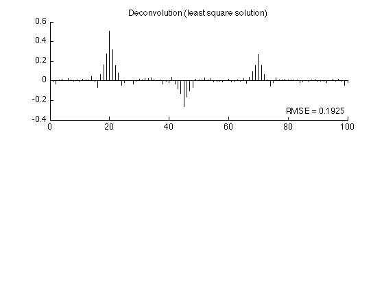
Find the least square solution to the deconvolution problem.
lambda = 0.4;                                       % lambda : regularization parameter

x_L2 = (H'*H + lambda*speye(N)) \ (H' * y);         % x_L2 : least square solution

rmse_L2 = sqrt(mean((x_L2 - s).^2));
fprintf('Least square solution: RMSE = %f\n', rmse_L2);

figure(2)
clf
subplot(2,1,1)
stem(x_L2, 'marker', 'none')
box off
title('Deconvolution (least square solution)');
axnote(sprintf('RMSE = %.4f', rmse_L2))
printme('L2')
Least square solution: RMSE = 0.192453
Verify banded system solver
Verify that MATLAB calls LAPACKS's fast algorithm for solving banded systems
spparms('spumoni', 3);      % Set sparse monitor flag to obtain diagnostic output

x_L2 = (H'*H + lambda*speye(N)) \ (H' * y);         % x_L2 : least square solution

%  Diagnostic output:
%
% sp\: bandwidth = 3+1+3.
% sp\: is A diagonal? no.
% sp\: is band density (1.00) > bandden (0.50) to try banded solver? yes.
% sp\: is LAPACK's banded solver successful? yes.

spparms('spumoni', 0);      % Reset sparse monitor flag to no diagnostic output
sp\: bandwidth = 3+1+3.
sp\: is A diagonal? no.
sp\: is band density (1.00) > bandden (0.50) to try banded solver? yes.
sp\: is LAPACK's banded solver successful? yes.
Sparse deconvolution - L1 norm penalty
The penalty function is phi(x) = lam abs(x)
T = 3 * sigma * sqrt(sum(abs(h).^2));   % T : threshold using '3-sigma' rule

lam = T;
Nit = 50;

phi_L1 = @(x) lam * abs(x);
wfun_L1 = @(x) abs(x)/lam;
dphi_L1 = @(x) lam * sign(x);

[x1, cost1] = deconv_MM(y, phi_L1, wfun_L1, H, Nit);

rmse1 = sqrt(mean((x1 - s).^2));
fprintf('L1 norm solution: RMSE = %f\n', rmse1);
L1 norm solution: RMSE = 0.034072
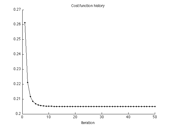
Display cost function history
figure(1)
clf
plot(1:Nit, cost1, '.-')
title('Cost function history');
xlabel('Iteration')
xlim([0 Nit])
box off
printme('CostFunction_L1')
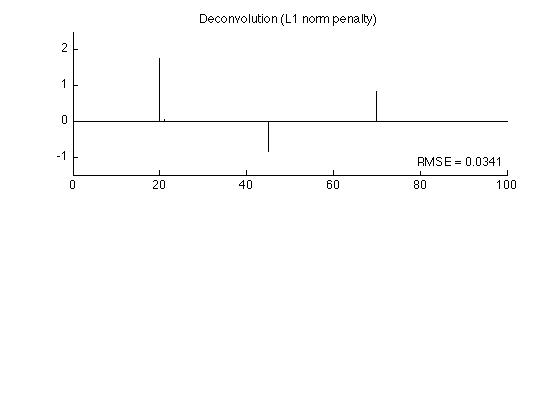
The L1 solution is quite similar to the original signal (much more so than the least square solution).
figure(2)
clf
subplot(2,1,1)
stem(x1, 'marker', 'none')
box off
ylim(ylim1);
title('Deconvolution (L1 norm penalty)');
axnote(sprintf('RMSE = %.4f', rmse1))
printme('L1')
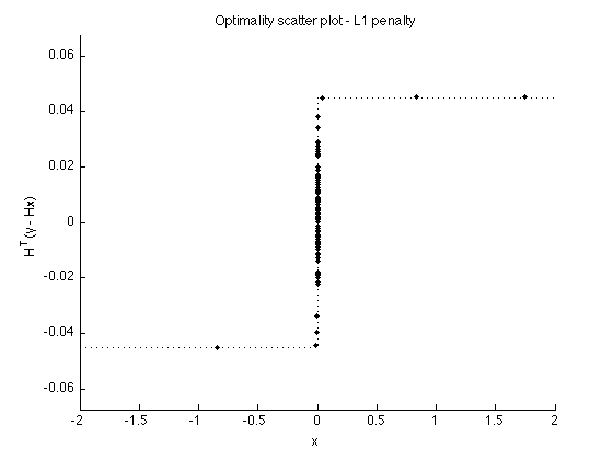
Verify optimality conditions
v1 = H'*(y-H*x1);

t = [linspace(-2, -eps, 100) linspace(eps, 2, 100)];

figure(1)
clf
plot(x1, v1, '.')
line(t, dphi_L1(t), 'linestyle', ':')
box off
ylim([-1 1]*lam*1.5)
xlabel('x')
ylabel('H^T(y - Hx)')
title('Optimality scatter plot - L1 penalty');

printme('scatter_L1')
Sparse deconvolution - nn garrote penalty
The penalty function corresponds to the nn garrote shrinkage function.
dphi = @(x) 0.5 * (- abs(x) + sqrt( x.^2 + 4*T^2 ) ) .* sign(x);

phi = @(x) T^2*asinh(abs(x)/(2*T)) +0.25 * (abs(x).*sqrt(4*T^2+x.^2)-x.^2) ;

wfun = @(x) 1/(2*T^2) * abs(x) .* ( sqrt(x.^2 + 4*T^2) + abs(x) );  % x / dphi(x)

[x2, cost2] = deconv_MM(y, phi, wfun, H, Nit);

rmse2 = sqrt(mean((x2 - s).^2));
fprintf('nn-garrote solution: RMSE = %f\n', rmse2);
nn-garrote solution: RMSE = 0.004564
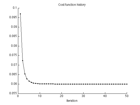
Display cost function history
figure(1)
clf
plot(1:Nit, cost2, '.-')
title('Cost function history');
xlabel('Iteration')
xlim([0 Nit])
box off
printme('CostFunction_garrote')
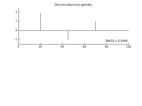
figure(2)
clf
subplot(2,1,1)
stem(x2, 'marker', 'none')
box off
ylim(ylim1);
title('Deconvolution (nn-garrote)');
axnote(sprintf('RMSE = %.4f', rmse2))
printme('garrote')
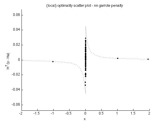
Verify (local) optimality conditions
v2 = H'*(y-H*x2);

figure(1)
clf
plot(x2, v2, '.')
line(t, dphi(t), 'linestyle', ':')
box off
ylim([-1 1]*T*1.5)
xlim(t([1 end]))
xlabel('x')
ylabel('H^T(y - Hx)')
title('(local) optimality scatter plot - nn garrote penalty');
printme('scatter_garrote')
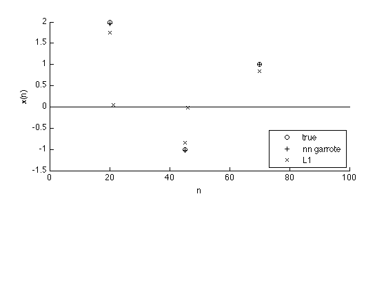
Comparison
The nn garrote penalty is more accurate than the L1 norm penalty. The result obtained using the L1 norm penalty is attenuated compared with the true signal.
n = 1:N;

k = abs(s) > 1e-5;
k1 = abs(x1) > 1e-5;
k2 = abs(x2) > 1e-5;

figure(1)
clf
subplot(3,1,[1 2])
plot(n(k), s(k), 'o')
hold on
plot(n(k2), x2(k2),'+', n(k1), x1(k1),'x')
line([0 N], [0 0])
hold off
xlim([0 N])
legend('true', 'nn garrote', 'L1', 'location', 'se')
box off
xlabel('n')
ylabel('x(n)')
printme('compare')