Linear prediction by least squares

The example illustrates the prediction of data using a linear predictor. The coefficients of the linear predictor are obtained by least squares.

Ivan Selesnick
selesi@poly.edu

Contents

Start

clear
close all

Load data

load data.txt;
whos

y = data;         % data value

  Name        Size            Bytes  Class     Attributes

  data      100x1               800  double              

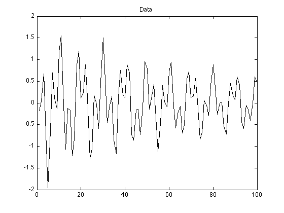
Display data

figure(1)
clf
plot(y)
title('Data')

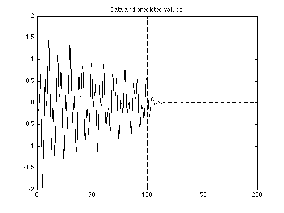
Linear predictor coefficients (2)

N = length(y);
H = [y(2:N-1) y(1:N-2)];        % H : rectangular matrix
b = y(3:N);                     % b : right-hand side of linear system of equations
a = (H' * H) \ (H' * b)         % a : coefficients of linear predictor

a =

    0.5648
   -0.5623

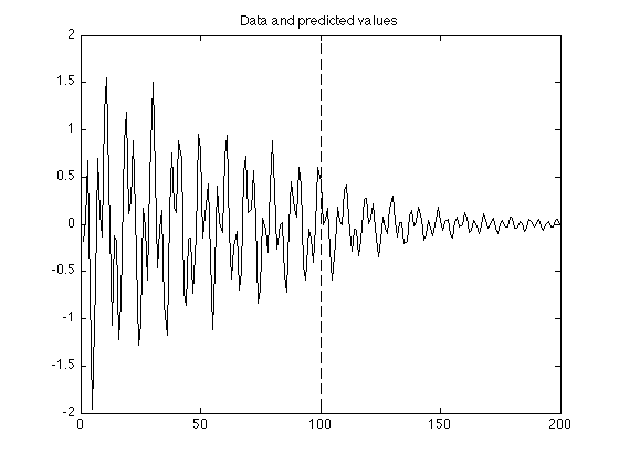
L = 100;                        % L : number of values to predict
g = [y; zeros(L, 1)];           % g : extended array (use first N samples to predict later samples)
for i = N+1:N+L
    g(i) = a(1) * g(i-1) + a(2) * g(i-2);    % linear prediction
end

figure(1)
clf
plot(g)
line([N N], [-2 2], 'linestyle', '--')
title('Data and predicted values')

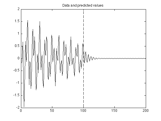
Linear predictor coefficients (3)

N = length(y);
H = [y(3:N-1) y(2:N-2) y(1:N-3)];
b = y(4:N);
a = (H' * H) \ (H' * b)         % a : coefficients of linear predictor

a =

    0.8777
   -0.8764
    0.5654

g = [y; zeros(L, 1)];
for i = N+1:N+L
    g(i) = a(1) * g(i-1) + a(2) * g(i-2) + a(3) * g(i-3);
end

figure(1)
clf
plot(g)
line([N N], [-2 2], 'linestyle', '--')
title('Data and predicted values')

Linear predictor coefficients (4)

N = length(y);
H = [y(4:N-1) y(3:N-2) y(2:N-3) y(1:N-4)];
b = y(5:N);
a = (H' * H) \ (H' * b)

a =

    1.4150
   -1.6741
    1.3634
   -0.8999

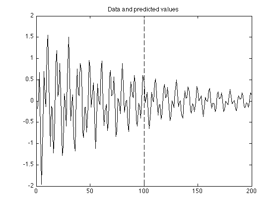
g = [y; zeros(L, 1)];
for i = N+1:N+L
    g(i) = a(1) * g(i-1) + a(2) * g(i-2) + a(3) * g(i-3) + a(4) * g(i-4);
end

figure(1)
clf
plot(g)
line([N N], [-2 2], 'linestyle', '--')
title('Data and predicted values')

Linear predictor coefficients (6)

N = length(y);
H = toeplitz(y(6:N-1), y(6:-1:1));    % Create H as a Toeplitz matrix (equivalent to above)
b = y(7:N);
a = (H' * H) \ (H' * b)

g = [y; zeros(L, 1)];
for i = N+1:N+L
    g(i) = a(1) * g(i-1) + a(2) * g(i-2) + a(3) * g(i-3) + a(4) * g(i-4) + a(5) * g(i-5) + a(6) * g(i-6);
end

figure(1)
clf
plot(g)
line([N N], [-2 2], 'linestyle', '--')
title('Data and predicted values')

a =

    0.0213
   -0.2861
   -0.1054
   -0.0536
   -0.4080
   -0.6518

Published with MATLAB® 7.8