Example: Dual basis pursuit (dual BP) with the DFT and STFT

Decompose a signal into two distinct signal components using dual basis pursuit (BP); i.e., MCA. In this example, the signal is the sum of a sinusoid and a pulse. The DFT and STFT are used for the two transforms.

Ivan Selesnick
November, 2013

Start
Create data
Define transforms
Verify transform A1
Verify transform A2
Peform signal separation using dual BP
Display signal components
Display sparse component coefficients
Save figure to file

Start

clear
% close all

I = sqrt(-1);

Create data

Sinusoid + pulse

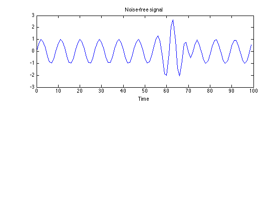
N = 100;                    % N : signal length
n = 0:N-1;

f1 = 0.112;
s1 = sin(2*pi*f1*n);      % s1 : complex sinusoid

f2 = 0.15;
K = 20;                     % K : duration of transient
M = 55;                     % M : start-time of transient
A = 3;
s2 = zeros(size(n));        % s2 : transient
s2(M+(1:K)) = A*sin(2*pi*f2*(1:K)) .* hamming(K)';

y = s1 + s2;                % Add two components

figure(1)
clf

subplot(2, 1, 1)
plot(n, y)
title('Noise-free signal')
xlabel('Time')

Define transforms

K = 200;                    % K : length of DFT
[A1, A1H, normA1] = MakeTransforms('DFT', N, K);

R = 16;                     % R : frame length
Nfft = 16;                  % Nfft : DFT length in STFT (Nfft >= R)
[A2, A2H, normA2] = MakeTransforms('STFT', N, [R Nfft]);

Reconstruction error = 0.000000
Energy ratio = 1.000000
Reconstruction error = 0.000000
Energy ratio = 1.000000

Verify transform A1

Verify properties of transform A1 (A AH = I)

% Verify perfect reconstruction property of transform 1 (A1*A1H = I)
c = A1H(y);
err = y - A1(c);
re = max(abs(err(:)));          % should be zero
fprintf('Reconstruction error = %f\n', re)

% Verify Parseval energy identity
E = sum(abs(y(:)).^2);
E1 = sum(abs(c(:)).^2);         % should be unity
fprintf('Energy ratio = %f\n', E1/E)

Reconstruction error = 0.000000
Energy ratio = 1.000000

Verify transform A2

Verify properties of transform A2 (A AH = I)

% Verify perfect reconstruction property of transform 2 (A2*A2H = I)
c = A2H(y);
err = y - A2(c);
re = max(abs(err(:)));          % should be zero
fprintf('Reconstruction error = %f\n', re)

% Verify Parseval energy identity
E = sum(abs(y(:)).^2);
E1 = sum(abs(c(:)).^2);         % should be unity
fprintf('Energy ratio = %f\n', E1/E)

Reconstruction error = 0.000000
Energy ratio = 1.000000

Peform signal separation using dual BP

Use 'dualBP' (dual basis pursuit) to separate the signal into two components.

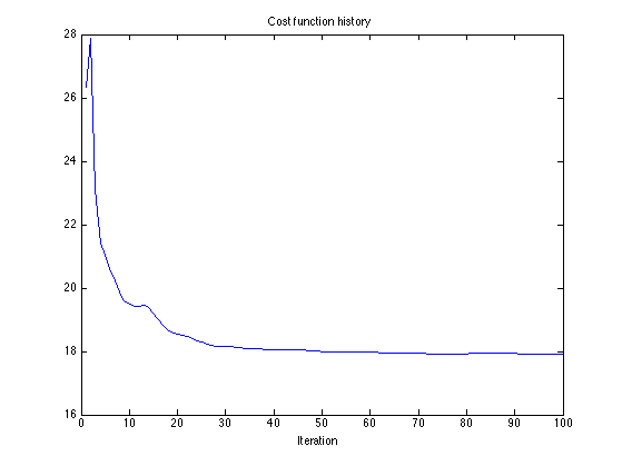
% Algorithm parameters
theta = 0.5;              % theta : trade-off parameter (0 < theta < 1)
Nit = 100;                % Nit : number of iterations
mu = 1;                   % mu : ADMM parameter

[x1, x2, c1, c2, cost] = dualBP(y, A1, A1H, A2, A2H, theta, mu, Nit);

% Display cost function history
figure(1)
clf
plot(cost)
xlim([0 Nit])
title('Cost function history')
xlabel('Iteration')

Display signal components

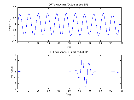
figure(1)
clf

subplot(2, 1, 1)
plot(n, real(x1))
title('DFT component [Output of dual BP]');
xlabel('Time')
ylabel('real( A1 c1)')

subplot(2, 1, 2)
plot(n, real(x2))
title('STFT component [Output of dual BP]');
xlabel('Time')
ylabel('real( A2 c2)')

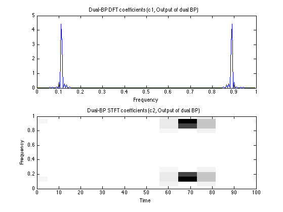
Display sparse component coefficients

f = (0:K-1)/K;          % f : frequency axis

tt = R/2 * ( (0:size(c2, 2)) - 1 );  % tt : time axis for STFT

figure(2)
clf

subplot(2, 1, 1)
plot(f, abs(c1))
title('Dual-BP DFT coefficients (c1, Output of dual BP)')
xlabel('Frequency')

subplot(2, 1, 2)
imagesc(tt, [0 1], abs(c2))
xlim([0 N])
ylim([0 1])
axis xy
title('Dual-BP STFT coefficients (c2, Output of dual BP)')
xlabel('Time')
ylabel('Frequency')

cm = colormap(gray);                % cm : colormap for STFT
cm = cm(end:-1:1, :);
colormap(cm)

Save figure to file

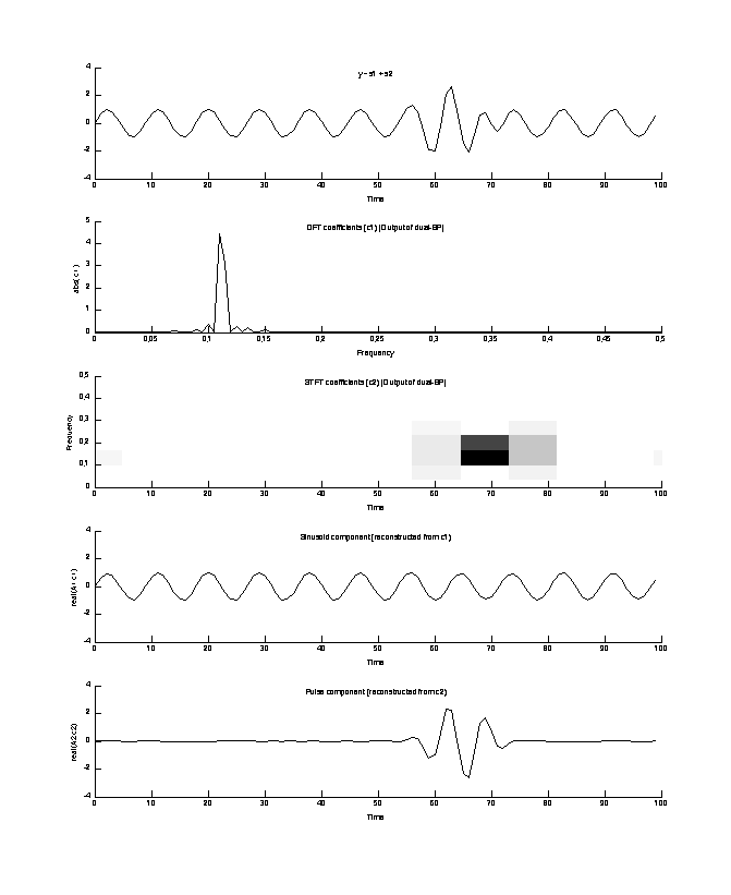
MyGraphPrefs('on')

figure(4)
clf

ylim1 = 4*[-1 1];

subplot(5, 1, 1)
line(n, y)
mytitle('y = s1 + s2');
xlabel('Time')
ylim(ylim1)

% Display sparse component coefficients

subplot(5, 1, 2)
line(f, abs(c1), 'marker', '.')
mytitle('DFT coefficients (c1) [Output of dual-BP]');
xlabel('Frequency')
ylabel('abs( c1 )')
xlim([0 0.5])

subplot(5, 1, 3)
imagesc(tt, [0 1], abs(c2))
xlim([0 N])
ylim([0 0.5])
axis xy
mytitle('STFT coefficients (c2) [Output of dual-BP]');
xlabel('Time')
ylabel('Frequency')
colormap(cm)
box off

% Dispaly signal components

subplot(5, 1, 4)
line(n, real(x1))
mytitle('Sinusoid component (reconstructed from c1)');
ylabel('real(A1 c1)')
xlabel('Time')
ylim(ylim1)

subplot(5, 1, 5)
line(n, real(x2))
ylim(ylim1)
mytitle('Pulse component (reconstructed from c2)');
ylabel('real(A2 c2)')
xlabel('Time')


% print figure to pdf file
orient tall
print -dpdf figures/dualBP_example1

% print figure to eps file
set(gcf, 'PaperPosition', [1 1 4.7 9])
print -deps figures_eps/dualBP_example1

MyGraphPrefs('off')