Example: Dual basis pursuit denoising (dual BPD) with the DFT and STFT

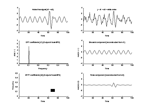
Decompose a signal into two distinct signal components using dual basis pursuit denoising (dual BPD); i.e., MCA. In this example, the data is the sum of a sinusoid, a pulse, and white noise. The DFT and STFT are used for the two transforms.

Ivan Selesnick
November, 2013
Revised January, 2014

Start
Create test data
Define transforms
Peform signal separation using dual BPD
Display signal components
Display sparse component coefficients
Optimality scatter plot (component 1)
Optimality scatter plot (component 2)
Save figure to file
Animate: vary lambda

Start

clear
% close all

I = sqrt(-1);

Create test data

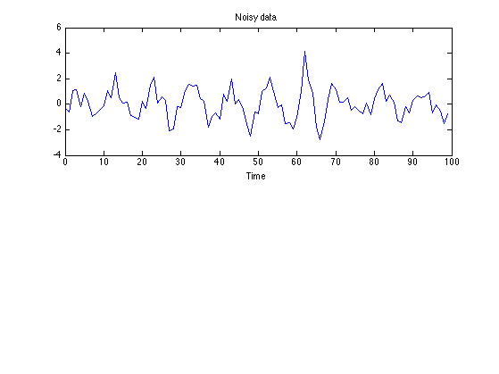
Sinusoid + pulse + white noise

N = 100;                    % N : signal length
n = 0:N-1;

f1 = 0.1;
s1 = sin(2*pi*f1*n);      % s1 : sinusoid

f2 = 0.15;
K = 20;                     % K : duration of pulse
M = 55;                     % M : start-time of pulse
A = 3;
s2 = zeros(size(n));        % s2 : pulse
s2(M+(1:K)) = A*sin(2*pi*f2*(1:K)) .* hamming(K)';

randn('state', 0);          % set state for reproducibility of example

sigma = 1;                  % sigma : noise standard deviation
w = sigma/sqrt(2) * randn(1, N);
                            % w : white Gaussian noise

y = s1 + s2 + w;            % y : two components plus noise

figure(1)
clf

subplot(2, 1, 1)
plot(n, y)
title('Noisy data')
xlabel('Time')

Define transforms

Nfft1 = 256;
[A1, A1H, normA1] = MakeTransforms('DFT', N, Nfft1);

R = 16;         % R : frame length
Nfft2 = 16;      % Nfft2 : FFT length in STFT (Nfft >= R)
[A2, A2H, normA2] = MakeTransforms('STFT', N, [R Nfft2]);

Reconstruction error = 0.000000
Energy ratio = 1.000000
Reconstruction error = 0.000000
Energy ratio = 1.000000

Peform signal separation using dual BPD

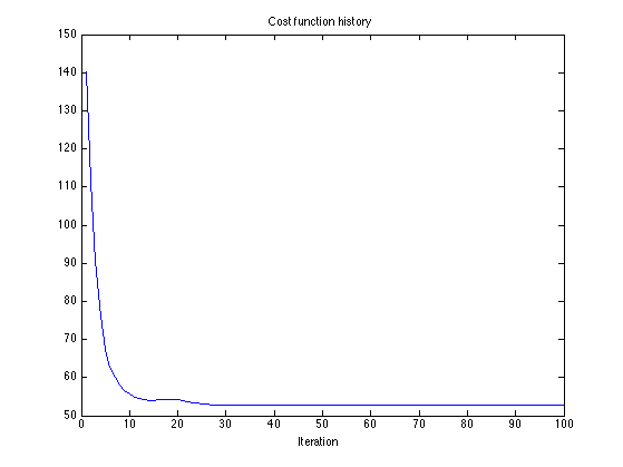
% Algorithm parameters
beta = 2.5;
lam1 = beta * sigma * normA1;
lam2 = beta * sigma * normA2;

Nit = 100;                  % Nit : number of iterations
mu = 1.0;                   % mu : ADMM parameter

[x1, x2, c1, c2, cost] = dualBPD(y, A1, A1H, A2, A2H, lam1, lam2, mu, Nit);

% Display cost function history
figure(1)
clf
plot(cost)
title('Cost function history')
xlabel('Iteration')

Display signal components

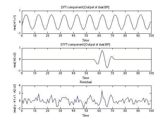
r = y - x1 - x2;        % residual

% DFT component
subplot(3, 1, 1)
plot(n, real(x1))
title('DFT component [Output of dual BP]');
xlabel('Time')
ylabel('real( A1 c1)')

% STFT component
subplot(3, 1, 2)
plot(n, real(x2))
title('STFT component [Output of dual BP]');
xlabel('Time')
ylabel('real( A2 c2)')

% residual
subplot(3, 1, 3)
plot(n, real(y - x1 - x2))
title('Residual');
xlabel('Time')
ylabel('real( y - A1 c1 - A2 c2)')

Display sparse component coefficients

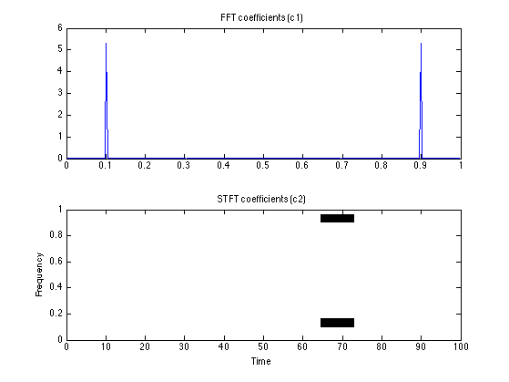
figure(1)
clf

f = (0:Nfft1-1)/Nfft1;

subplot(2, 1, 1)
plot(f, abs(c1))
title('FFT coefficients (c1)')

tt = R/2 * ( (0:size(c2, 2)) - 1 );  % tt : time axis for STFT

subplot(2, 1, 2)
imagesc(tt, [0 1], abs(c2))
axis xy
xlim([0 N])
ylim([0 1])
title('STFT coefficients (c2)')
xlabel('Time')
ylabel('Frequency')

cm = colormap(gray);                % cm : colormap for STFT
cm = cm(end:-1:1, :);
colormap(cm)

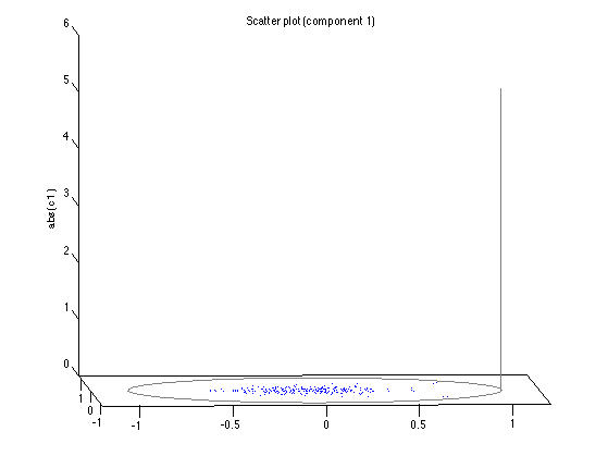
Optimality scatter plot (component 1)

g1 = A1H(y - A1(c1) - A2(c2)) .* exp(-I*angle(c1)) / lam1;

c1max = max(abs(c1(:)));

theta = linspace(0, 2*pi, 200);

figure(2)
clf
plot3( real(g1), imag(g1), abs(c1), '.')
zlabel('abs( c1 )')
% xlabel('Re(A1^H(y - A1 c1 - A2 c2) exp(-j\anglec))/\lambda_1')
% ylabel('Im(A1^H(y - A1 c1 - A2 c2) exp(-j\anglec))/\lambda_1')
title('Scatter plot (component 1)')
grid off
box off
line( cos(theta), sin(theta), 'color', [1 1 1]*0.5)
line([1 1], [0 0], [0 c1max],  'color', [1 1 1]*0.5)
xlim([-1 1] * 1.2)
ylim([-1 1] * 1.2)
line([-1 1]*1.2, [1 1]*1.2, 'color', 'black')
line([1 1]*1.2, [-1 1]*1.2, 'color', 'black')

% Animate: vary view orientation
az = -36;
for el = [40:-1:5]
    view([az el])
    drawnow
end
for az = [-36:-3]
    view([az el])
    drawnow
end

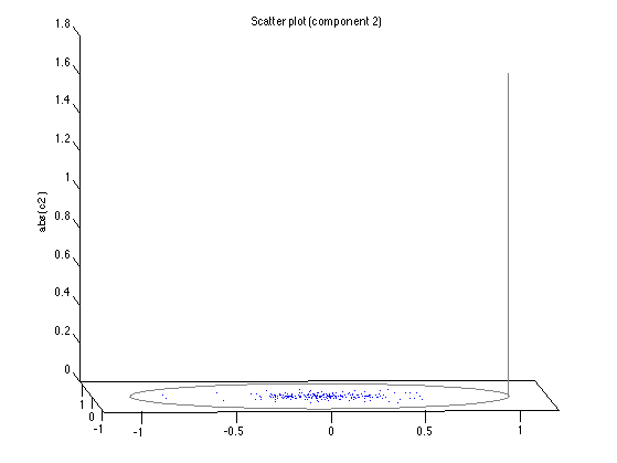
Optimality scatter plot (component 2)

g2 = A2H(y - A1(c1) - A2(c2)) .* exp(-I*angle(c2)) / lam2;

c2max = max(abs(c2(:)));

figure(2)
clf
plot3( real(g2(:)), imag(g2(:)), abs(c2(:)), '.')
zlabel('abs( c2 )')
% xlabel('Re(A2^H(y - A1 c1 - A2 c2) exp(-j\anglec))/\lambda_2')
% ylabel('Im(A2^H(y - A1 c1 - A2 c2) exp(-j\anglec))/\lambda_2')
title('Scatter plot (component 2)')
grid off
box off
line( cos(theta), sin(theta), 'color', [1 1 1]*0.5)
line([1 1], [0 0], [0 c2max],  'color', [1 1 1]*0.5)
xlim([-1 1] * 1.2)
ylim([-1 1] * 1.2)
line([-1 1]*1.2, [1 1]*1.2, 'color', 'black')
line([1 1]*1.2, [-1 1]*1.2, 'color', 'black')

% Animate: vary view orientation
az = -36;
for el = [40:-1:5]
    view([az el])
    drawnow
end
for az = [-36:-3]
    view([az el])
    drawnow
end

Save figure to file

MyGraphPrefs('on')

figure(3)
clf

ylim1 = [-4 4];

% Noise-free signal

subplot(3, 2, 1)
line(n, s1+s2)
mytitle('Noise-free signal (s1 + s2)');
xlabel('Time')
ylim(ylim1)

% Noisy data

subplot(3, 2, 2)
line(n, y)
mytitle('y = s1 + s2 + white noise');
xlabel('Time')
ylim(ylim1)

% Coefficients (output of dual BPD)

subplot(3, 2, 3)
line(f, abs(c1), 'marker', '.')
mytitle('DFT coefficients (c1) [Output of dual-BPD]');
xlabel('Frequency')
ylabel('abs( c1 )')
xlim([0 0.5])
ylim([0 7])

subplot(3, 2, 5)
imagesc(tt, [0 1], abs(c2))
axis xy
xlim([0 N])
ylim([0 0.5])
mytitle('STFT coefficients (c2) [Output of dual-BPD]');
xlabel('Time')
ylabel('Frequency')
colormap(cm)
box off

% Signals (reconstructed from dual-BPD coefficients)

subplot(3, 2, 4)
line(n, real(x1))
mytitle('Sinusoid component (reconstructed from c1)');
ylabel('real(A1 c1)')
xlabel('Time')
ylim(ylim1)

subplot(3, 2, 6)
line(n, real(x2))
ylim(ylim1)
mytitle('Pulse component (reconstructed from c2)');
ylabel('real(A2 c2)')
xlabel('Time')


% print figure to pdf file
orient landscape
print -dpdf figures/dualBPD_example1

% print figure to eps file
orient portrait
set(gcf, 'PaperPosition', [1 1 7.5 6])
print -deps figures_eps/dualBPD_example1

MyGraphPrefs('off')

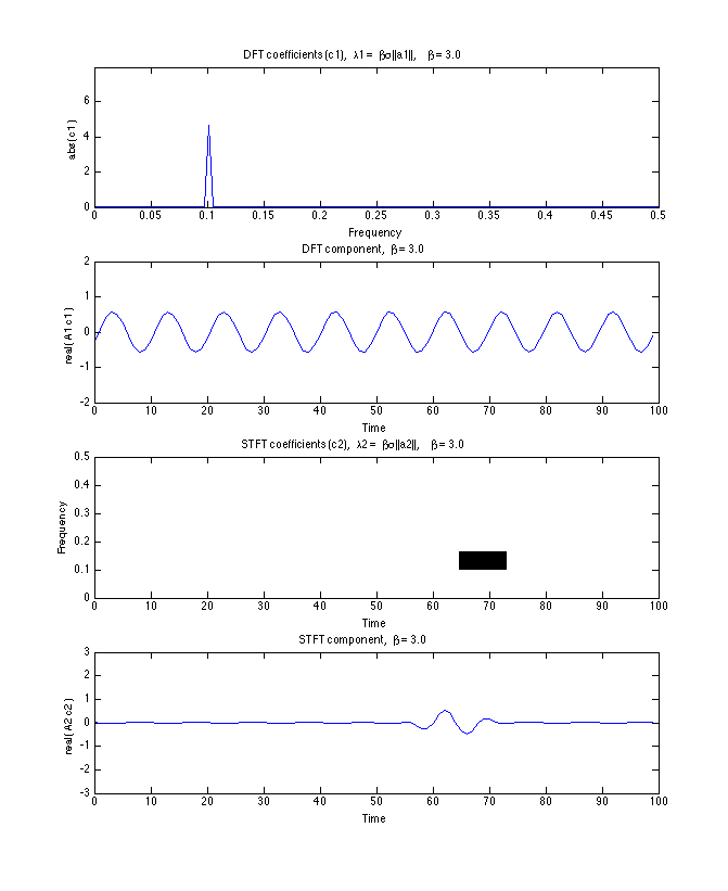
Animate: vary lambda

figure(4)
clf

% Modify figure size (try to make larger than default)
ss = get(0, 'screensize');
set(gcf, 'position', round([0.2*ss(3), 0.1*ss(4), 0.4*ss(3), 0.8*ss(4)]));
% [left bottom width height]

for beta = 0.1:0.1:3

    lam1 = beta * sigma * normA1;
    lam2 = beta * sigma * normA2;
    [x1, x2, c1, c2, cost] = dualBPD(y, A1, A1H, A2, A2H, lam1, lam2, mu, Nit);

    subplot(4, 1, 1)
    plot(f, abs(c1), '.-')
    title(sprintf('DFT coefficients (c1), \\lambda1 = \\beta\\sigma ||a1||, \\beta = %.1f', beta));
    ylabel('abs( c1 )')
    xlabel('Frequency')
    xlim([0 0.5])
    ylim([0 1.5*c1max])

    subplot(4, 1, 2)
    plot(n, real(x1))
    ylim([-1 1]*2)
    title(sprintf('DFT component, \\beta = %.1f', beta));
    ylabel('real( A1 c1 )')
    xlabel('Time')

    subplot(4, 1, 3)
    imagesc(tt, [0 1], abs(c2))
    colormap(cm)
    axis xy
    xlim([0 N])
    ylim([0 0.5])
    title(sprintf('STFT coefficients (c2), \\lambda2 = \\beta\\sigma ||a2||, \\beta = %.1f', beta));
    xlabel('Time')
    ylabel('Frequency')

    subplot(4, 1, 4)
    plot(n, real(x2))
    ylim([-1 1]*3)
    title(sprintf('STFT component, \\beta = %.1f', beta));
    xlabel('Time')
    ylabel('real( A2 c2 )')

    drawnow

end