Example: Basis pursuit denoising (BPD) with the DFT

Estimation of sinusoids in white Gaussian noise

Contents

Misc

clear
close all

I = sqrt(-1);

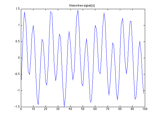
Make signal

N = 100;                   % N : signal length
n = 0:N-1;

f1 = 0.05;
f2 = 0.14;
s = 0.5*sin(2*pi*f1*n) + sin(2*pi*f2*n - pi/3);
% s : sinusoid

figure(1)
clf
plot(n, s)
title('Noise-free signal [s]')

Define transform

zero-padded DFT

Nfft = 256;

[A, AH, normA] = MakeTransforms('DFT', N, Nfft);

Reconstruction error = 0.000000
Energy ratio = 1.000000

Validate normA calculation

% imp : an impulse in transform domain
imp = zeros(1, Nfft);
n0 = 10;
imp(n0) = 1;

[normA norm(A(imp))]   % should be same

ans =

    0.6250    0.6250

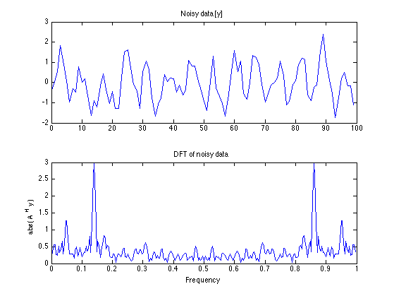
Make noisy data

sigma = 0.5;

randn('state', 1); % set state for reproducibility of example

y = s + sigma * randn(size(s));

f = (0:Nfft-1)/Nfft;        % f : frequency axis

figure(1)
clf

subplot(2, 1, 1)
plot(n, y)
title('Noisy data [y]')

subplot(2, 1, 2)
plot(f, abs( AH(y) ))
title('DFT of noisy data')
ylabel('abs( A^H y )')
xlabel('Frequency')

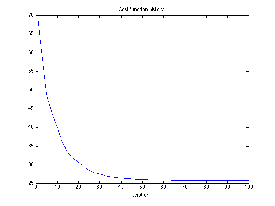
Solve BPD problem

beta = 3;
beta = 2.5;
lam = beta * sigma * normA;

mu = 0.1;
Nit = 100;

[c, cost] = BPD(y, A, AH, lam, mu, Nit);

x = A(c);

% Display cost function history to observe convergence of algorithm.
figure(1)
clf
plot(cost)
title('Cost function history')
xlabel('Iteration')

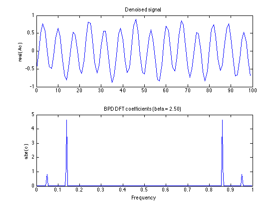
Display denoised signal

figure(1)
clf

subplot(2, 1, 1)
plot(n, real(x))
title('Denoised signal')
ylabel('real( Ac )')

subplot(2, 1, 2)
plot(f, abs(c), '.-')
title(sprintf('BPD DFT coefficients (beta = %.2f)', beta));
ylabel('abs( c )')
xlabel('Frequency')

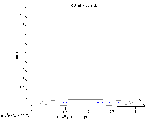
Optimality scatter plot

I = sqrt(-1);
g = (1/lam) * AH(y - A(c)) .* exp(-I*angle(c));

cmax = max(abs(c));

figure(2)
clf
plot3( real(g), imag(g), abs(c), '.')
zlabel('abs( c )')
xlabel('Re(A^H(y - A c) e^{-j\anglec})/\lambda')
ylabel('Im(A^H(y - A c) e^{-j\anglec})/\lambda')
title('Optimality scatter plot')
grid off
theta = linspace(0, 2*pi, 200);
line( cos(theta), sin(theta), 'color', [1 1 1]*0.5)
line([1 1], [0 0], [0 cmax],  'color', [1 1 1]*0.5)
xm = 1.2;
xlim([-1 1]*xm)
ylim([-1 1]*xm)
line([-1 1]*xm, [1 1]*xm, 'color', 'black')
line([1 1]*xm, [-1 1]*xm, 'color', 'black')
box off

% Animate: vary view orientation
az = -36;
for el = [40:-1:5]
    view([az el])
    drawnow
end
for az = [-36:-3]
    view([az el])
    drawnow
end

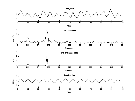
Save figure to file

MyGraphPrefs('on')

figure(3)
clf

subplot(4, 1, 1)
line(n, y)
mytitle('Noisy data');
ylabel('y')
xlabel('Time')
ylim([-3 3])

subplot(4, 1, 2)
line(f, abs(AH(y) ))
mytitle('DFT of noisy data');
ylabel('abs( A^H y )')
xlabel('Frequency')
xlim([0 0.5])

subplot(4, 1, 3)
line(f, abs(c), 'marker', '.')
% title('DFT coefficients [Output of BPD]');
mytitle(sprintf('BPD DFT (beta = %.2f)', beta));
ylabel('abs( c )')
xlabel('Frequency')
xlim([0 0.5])

subplot(4, 1, 4)
line(n, real(A(c)))
mytitle('Denoised data');
ylabel('real( Ac )')
xlabel('Time')
ylim([-3 3])

% print figure to pdf file
orient tall
print -dpdf figures/BPD_example_dft

% print figure to eps file
set(gcf, 'PaperPosition', [1 1 4 7])
print -deps figures_eps/BPD_example_dft

MyGraphPrefs('off')

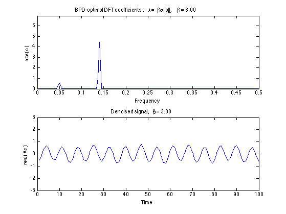
Animate: vary lambda

for beta = 0.1:0.1:3

    lam = beta * sigma * normA;
    [c, cost] = BPD(y, A, AH, lam, mu, Nit);
    x = A(c);

    figure(10)
    clf

    subplot(2, 1, 1)
    plot(f, abs(c), '.-')
    xlim([0 0.5])
    ylim([0 1.5*cmax])
    title(sprintf('BPD-optimal DFT coefficients : \\lambda = \\beta\\sigma ||a||, \\beta = %.2f', beta));
%     title(sprintf('\\beta = %.2f; \\lambda = \\beta \\sigma ||a||', beta));
    ylabel('abs( c )')
    xlabel('Frequency')

    subplot(2, 1, 2)
    plot(real(x))
    ylim([-3 3])
    title(sprintf('Denoised signal, \\beta = %.2f', beta));
    ylabel('real( Ac )')
    xlabel('Time')

    drawnow

end

Published with MATLAB® 7.12