Smooth Wavelet Tight Frames with Zero Moments

Example 3: K₀ = 7, K₁ = K₂ = 3

There are 8 different minimal-length solutions. The solutions in terms of radicals, obtained using Gröbner bases, are tabulated in the MATLAB program k733.m. The numerical solutions are tabulated in the file k733.float. The system k733(1) is shown in this figure. All eight solutions are shown together on another page.

The filters h0, h1, h2 were found by first converting the nonlinear design equations (eqs) into a degree Gröbner basis (gb.dp), and converting that into a lexical Gröbner basis (gb.lp). Note that these Gröbner bases are quite large. Moroever, with the ordering used, the Gröbner basis gb.lp does not factor. We found that by changing ordering of variables, the Gröbner basis does factor. Specifically, the lexical Gröbner basis (gb.lp.b0) computed from gb.lp with the new ordering, factors into 4 separate parts (gb.lp.b0.fact.1, gb.lp.b0.fact.2, gb.lp.b0.fact.3, gb.lp.b0.fact.4). Changing the ordering for each Gröbner basis again, we obtain 4 lexical Gröbner bases which are more compact (gb.lp.fact.1, gb.lp.fact.2, gb.lp.fact.3, gb.lp.fact.4).

The Gröbner bases indicate that there are 64 solutions to the nonlinear design equations (16 solutions from each of gb.lp.fact.*). However, excluding time-reversal and negation, there are 8 distinct solutions (2 solutions from each of gb.lp.fact.*). The solutions derived from these 4 lexical Gröbner bases are tabulated in the MATLAB programs c1.m, c2.m, c3.m, c4.m.

We also provide for this example the programs for reproducing these steps: the Maple program (setup) for generating the equations , the Singular program (sfile) for obtaining the Gröbner bases, and the Maple program (result) for solving the Gröbner bases. Executing these programs in sequence will regenerate the Gröbner bases and create the four MATLAB programs c1.m, c2.m, c3.m, c4.m containing the solutions, which were combined into k733.m. Note, however, that the Gröbner basis computations took us several days on a Sun Ultra 2. But the advantage of Gröbner bases are that the results are exact.

K₀ = 7, K₁ = K₂ = 3. Solution 1.

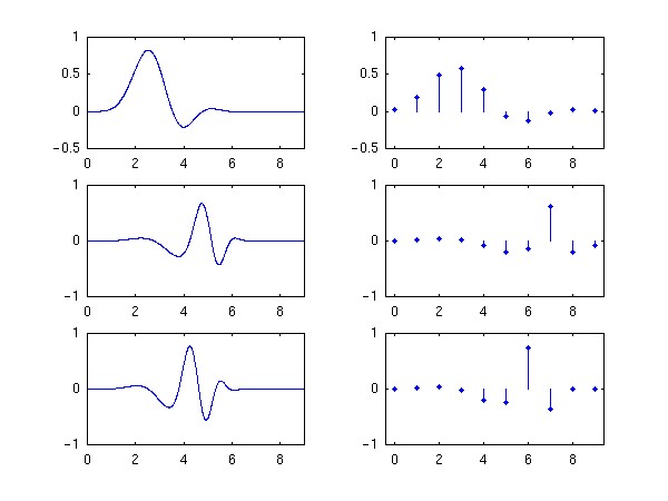
The scaling and wavelet functions are on the right. The scaling and wavelet filters are on the left.