1-D Discrete Wavelet Transform

1. 2-Channel Perfect Reconstruction Filter Bank

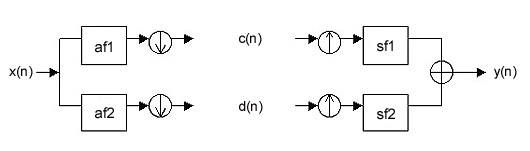
The analysis filter bank decomposes the input signal x(n) into two subband signals, c(n) and d(n). The signal c(n) represents the low frequency (or coarse) part of x(n), while the signal d(n) represents the high frequency (or detail) part of x(n). The analysis filter bank first filters x(n) using a lowpass and a highpass filter. We denote the lowpass filter by af1 (analysis filter 1) and the highpass filter by af2 (analysis filter 2). As shown in the figure, the output of each filter is then down-sampled by 2 to obtain the two subband signals, c(n) and d(n).

The Matlab program below, afb.m, implements the analysis filter bank. The program uses the Matlab function upfirdn (in the Signal Processing Toolbox) to implement the filtering and downsampling.

function [lo, hi] = afb(x, af)

% [lo, hi] = afb(x, af)
%
% Analysis filter bank
% x -- N-point vector (N even); the resolution should be 2x filter length
%
% af  -- analysis filters
% af(:, 1): lowpass filter (even length)
% af(:, 2): highpass filter (even length)
%
% lo: Low frequency
% hi: High frequency
%

N = length(x);
L = length(af)/2;
x = cshift(x,-L);

% lowpass filter
lo = upfirdn(x, af(:,1), 1, 2);
lo(1:L) = lo(N/2+[1:L]) + lo(1:L);
lo = lo(1:N/2);

% highpass filter
hi = upfirdn(x, af(:,2), 1, 2);
hi(1:L) = hi(N/2+[1:L]) + hi(1:L);
hi = hi(1:N/2);

The synthesis filter bank combines the two subband signals c(n) and d(n) to obtain a single signal y(n). The synthesis filter bank first up-samples each of the two subband signals. The signals are then filtered using a lowpass and a highpass filter. We denote the lowpass filter by sf1 (synthesis filter 1) and the highpass filter by sf2 (synthesis filter 2). The signals are then added together to obtain the signal y(n). If the four filters are designed so as to guarantee that the output signal y(n) equals the input signal x(n), then the filters are said to satisfy the perfect reconstruction condition. The Matlab program below, sfb.m, implements the synthesis filter bank.

function y = sfb(lo, hi, sf)

% y = sfb(lo, hi, sf)
%
% Synthesis filter bank
%
% lo - low frqeuency signal
% hi - high frequency signal
% sf - synthesis filters
% sf(:, 1) - lowpass filter (even length)
% sf(:, 2) - highpass filter (even length)
%
% y - output

N = 2*length(lo);
L = length(sf);
lo = upfirdn(lo, sf(:,1), 2, 1);
hi = upfirdn(hi, sf(:,2), 2, 1);
y = lo + hi;
y(1:L-2) = y(1:L-2) + y(N+[1:L-2]);
y = y(1:N);
y = cshift(y, 1-L/2);

There are many sets of filters that satisfy the perfect reconstruction conditions. One set of filters, from [AS-2001], is shown in the Table below. These filters are approximately symmetric.

  --------------------------------------------------------
      af1              af2            sf1              sf2
  --------------------------------------------------------
        0          -0.0112          0.0112               0
        0           0.0112          0.0112               0
  -0.0884           0.0884         -0.0884         -0.0884
   0.0884           0.0884          0.0884         -0.0884
   0.6959          -0.6959          0.6959          0.6959
   0.6959           0.6959          0.6959         -0.6959
   0.0884          -0.0884          0.0884          0.0884
  -0.0884          -0.0884         -0.0884          0.0884
   0.0112                0               0          0.0112
   0.0112                0               0         -0.0112
   --------------------------------------------------------
 

The following code fragment shows an example of how to use the Matlab functions, afb.m and sfb.m. This example verifies the perfect reconstruction property. First, we create a random input signal x of length 64. Then the analysis and synthesis filters are obtained with the Matlab function farras.m. The two subband signals (here called lo and hi) are computed with the function afb.m. The output signal y is then computed using the Matlab function sfb.m. The maximum value of the error x - y is computed, and it is equal to zero (within computer precision). This verifies the perfect reconstruction property.

>> [af, sf] = farras;        % analysis and synthesis filter
>> x = rand(1,64);           % create generic signal
>> [lo, hi] = afb(x, af);    % analysis filter bank
>> y = sfb(lo, hi, sf);      % synthesis filter bank
>> err = x - y;              % compute error signal
>> max(abs(err))             % verify that error is zero

ans =

  1.9096e-014 
  

A couple of remarks about the programs afb.m and sfb.m. Suppose the input signal x(n) is of length N. For convenience, we will like the subband signals c(n) and d(n) to each be of length N/2. However, these subband signals will exceed this length by L/2, where L is the length of the analysis filters.

To avoid this excessive length, the last L/2 samples of each subband signal is added to the first L/2 samples. This procedure (periodic extension) can create undesirable artifacts at the beginning and end of the subband signals, however, it is the most convenient solution. When the analysis and synthesis filters are exactly symmetric, a different procedure (symmetric extension) can be used, that avoids the artifacts associated with periodic extension.

A second detail also arises in the implementation of the perfect reconstruction filter bank. If all four filters are causal, then the output signal y(n) will be a translated (or circularly shifted) version of x(n). To avoid this, we perform a circular shift in both the analysis and synthesis filter banks. The circular shift is implemented with the Matlab function cshift.m.

2. Discrete Wavelet Transform (Iterated Filter Banks)

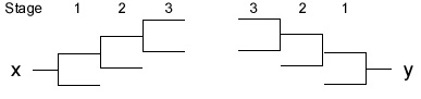
The discrete wavelet transform (DWT) gives a multiscale representation of a signal x(n). The DWT is implemented by iterating the 2-channel analysis filter bank described above. Specifically, the DWT of a signal is obtained by recursively applying the lowpass/highpass frequency decomposition to the lowpass output as illustrated in the diagram. The diagram illustrates a 3-scale DWT. The DWT of the signal x is the collection of subband signals. The inverse DWT is obtained by iteratively applying the synthesis filter bank.

The Matlab function dwt.m below computes the J-scale discrete wavelet transform w of the signal x. We use the cell array data structure of Matlab to store the subband signals. For j = 1..J, w{j} is the high frequency subband signal produced at stage j. w{J+1} is the low frequency subband signal produced at stage J.

function w = dwt(x, J, af)

% Discrete 1-D Wavelet Transform
%
% w = dwt(x, J, af)
% x  : 1-by-N data vector; the resolution should be 2^J times filter length
% J  : number of stages
% af : analysis filters
% af(:, 1) - lowpass filter
% af(:, 2) - highpass filter
%
% w{k} :
%    k = 1..J+1

for k = 1:J
    [x w{k}] = afb(x, af);
end
w{J+1} = x;

The inverse DWT is computed with the Matlab function idwt.m. The perfect reconstruction of the DWT is verified in the following example. First we create a random input signal x of length 64. Then the analysis and synthesis filters are obtained with the Matlab function farras.m. The 3-scale DWT is computed with the function dwt.m. The inverse DWT is then computed to get the signal y. As verified below, y = x within computer precision.

>> [af, sf] = farras;     % analysis and synthesis filter
>> x = rand(1,64);        % create generic signal
>> w = dwt(x,3,af);       % analysis filter banks (3 stages)
>> y = idwt(w,3,sf);      % synthesis filter banks (3 stages)
>> err = x-y;             % compute error signal
>> max(abs(err))          % verify that error is zero

ans =

  4.2633e-014
    

The wavelet associated with a set of synthesis filters can be computed using the following Matlab code fragment. In this example, we set all of the wavelet coefficients to zero, for the exception of one wavelet coefficient which is set to one. We then take the inverse wavelet transform.

>> [af, sf] = farras;     % analysis and synthesis filters
>> x=zeros(1,64);         % create zero signal 
>> w = dwt(x,3,af);       % analysis filter bank (3 stages)
>> w{3}(5)=1;             % set single coefficient to 1
>> y = idwt(w,3,sf);      % synthesis filter bank (3 stages)
>> plot(0:63,y);          % Plot the wavelet
>> axis([0 63 -0.5 0.5]);     
>> title('Standard 1-D wavelet') 
>> xlabel('t');                    
>> ylabel('\psi(t)');

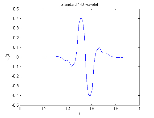
Other sets of filters will produce different wavelets.

Summary of programs:

1. farras.m - A set of perfect reconstruction filters
2. afb.m - Analysis filter bank
3. sfb.m - Synthesis filter bank
4. dwt.m - Forward wavelet transform
5. idwt.m - Inverse wavelet transform
6. cshift.m - Circular shift