2-D Dual-Tree Wavelet Transform

One of the advantages of the dual-tree complex wavelet transform is that it can be used to implement 2D wavelet transforms that are more selective with respect to orientation than is the separable 2D DWT.

There are two versions of the 2D dual-tree wavelet transform: the real 2-D dual-tree DWT is 2-times expansive, while the complex 2-D dual-tree DWT is 4-times expansive. Both types have wavelets oriented in six distinct directions. We describe the real version first.

1. Real 2-D Dual-tree Wavelet Transform

The real 2-D dual-tree DWT of an image x is implemented using two critically-sampled separable 2-D DWTs in parallel. Then for each pair of subbands we take the sum and difference. The following program, dualtree2D.m, computes the J-scale real 2-D dual-tree DWT of an image x.

function w = dualtree2D(x, J, Faf, af)

% 2D Dual-Tree Discrete Wavelet Transform
%
% w = dualtree2D(x, J, Faf, af)
% INPUT:
%    x   - 2-D signal
%    J   - number of stages
%    Faf - first stage filters
%    af  - filters for remaining stages
% OUPUT:
%    w{i}{1:J+1}: tree i wavelet coeffs (i = 1,2)

[x1 w{1}{1}] = afb2D(x, Faf{1});
for k = 2:J
    [x1 w{k}{1}] = afb2D(x1, af{1});
end
w{J+1}{1} = x1;

[x2 w{1}{2}] = afb2D(x, Faf{2});
for k = 2:J
    [x2 w{k}{2}] = afb2D(x2, af{2});
end
w{J+1}{2} = x2;

for k = 1:J
    for m = 1:3
        [w{k}{1}{m} w{k}{2}{m}] = pm(w{k}{1}{m},w{k}{2}{m});
    end
end

The wavelet coefficients w are stored as a cell array. For j = 1..J, k = 1..2, d = 1..3, w{j}{k}{d} are the wavelet coefficients produced at scale j and orientation (k,d). The image x is recovered from w using the inverse transform, implemented by idualtree2D.m. The perfect reconstruction property of the transform is illustrated in the following code fragment.

>> x = rand(256);
>> J = 3;
>> [Faf, Fsf] = FSfarras;
>> [af, sf] = dualfilt1;
>> w = dualtree2D(x, J, Faf, af);
>> y = idualtree2D(w, J, Fsf, sf);
>> err = x - y; max(max(abs(err)))

ans =

  2.8075e-008
  

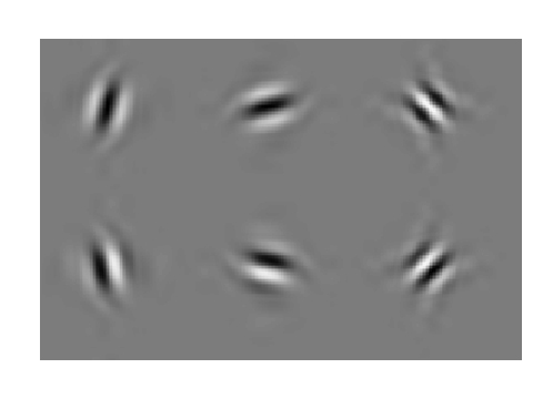
The six wavelets associated with the real 2D dual-tree DWT are illustrated in the following figures as gray scale images.

Note that each of the six wavelet are oriented in a distinct direction. Unlike the critically-sampled separable DWT, all of the wavelets are free of checker board artifact. Each subband of the 2-D dual-tree transform corresponds to a specific orientation. This figure was produced with the following Matlab program (dualtree2D_plots.m).

% dualtree2D_plots
% DISPLAY 2D WAVELETS OF dualtree2D.M

J = 4;
L = 3*2^(J+1);
N = L/2^J;
[Faf, Fsf] = FSfarras;
[af, sf] = dualfilt1;
x = zeros(2*L,3*L);
w = dualtree2D(x, J, Faf, af);
w{J}{1}{1}(N/2,N/2+0*N) = 1;
w{J}{1}{2}(N/2,N/2+1*N) = 1;
w{J}{1}{3}(N/2,N/2+2*N) = 1;
w{J}{2}{1}(N/2+N,N/2+0*N) = 1;
w{J}{2}{2}(N/2+N,N/2+1*N) = 1;
w{J}{2}{3}(N/2+N,N/2+2*N) = 1;
y = idualtree2D(w, J, Fsf, sf);

figure(1)
clf
imagesc(y);
axis equal
axis off
colormap(gray(128))

In this program, all of the wavelet coefficients are set to zero, for the exception of one wavelet coefficient in each of the six subbands. We then take the inverse wavelet transform.

2. Complex 2-D Dual-tree Wavelet Transform

The complex 2-D dual-tree DWT also gives rise to wavelets in six distinct directions, however, in this case there are two wavelets in each direction as will be illustrated below. In each direction, one of the two wavelets can be interpreted as the real part of a complex-valued 2D wavelet, while the other wavelet can be interpreted as the imaginary part of a complex-valued 2D wavelet. Because the complex version has twice as many wavelets as the real version of the transform, the complex version is 4-times expansive. The complex 2-D dual-tree is implemented as four critically-sampled separable 2-D DWTs operating in parallel. However, different filter sets are used along the rows and columns. As in the real case, the sum and difference of subband images is performed to obtain the oriented wavelets. The complex 2-D dual-tree DWT of an image x is computed by the following function, cplxdual2D.m.

function w = cplxdual2D(x, J, Faf, af)

% complex dual-tree 2D DWT
%
% w = cplxdual2D(x, J, Faf, af)
% x: 2-D signal
% J: number of stages
% Faf{i}: first stage filters for tree i
% af{i}:  filters for remaining stages on tree i
%
% Faf{i}(:,1), af{i}(:,1):   lowpass filter
% Faf{i}(:,2), af{i}(:, 2):  highpass filter 
%
% w: wavelet coefficients
%  w{1..J}{part}{d1}{d2}: 
%    scale = 1...J
%      part = 1 (real part), or part = 2 (imag part)
%      d1 = 1,2; d2 = 1,2,3 (orientations)
%  w{J+1}{m}{n}:
%      m = 1,2; n = 1,2 (lowpass subbands)
%      
% % Example:
% x = rand(256);
% J = 5;
% [Faf, Fsf] = FSfarras;
% [af, sf] = dualfilt1;
% w = cplxdual2D(x, J, Faf, af);
% y = icplxdual2D(w, J, Fsf, sf);
% err = x - y; max(max(abs(err)))

for m = 1:2
    for n = 1:2
        [lo w{1}{m}{n}] = afb2D(x, Faf{m}, Faf{n});
        for j = 2:J
            [lo w{j}{m}{n}] = afb2D(lo, af{m}, af{n});
        end
        w{J+1}{m}{n} = lo;
    end
end

for j = 1:J
    for m = 1:3
        [w{j}{1}{1}{m} w{j}{2}{2}{m}] = pm(w{j}{1}{1}{m},w{j}{2}{2}{m});
        [w{j}{1}{2}{m} w{j}{2}{1}{m}] = pm(w{j}{1}{2}{m},w{j}{2}{1}{m});
    end
end

The wavelet coefficients w are stored as a cell array. For j = 1..J, p = 1..2, k = 1..2, d = 1..3, w{j}{p}{k}{d} are the wavelet coefficients produced at scale j and orientation (k,d). With p = 1 we get the real part, with p = 2 we get the imaginary part. The image x is recovered from w using the inverse transform, implemented by icplxdual2D.m.The perfect reconstruction property of the transform is illustrated in the following code fragment.

>> x = rand(256);
>> J = 5;
>> [Faf, Fsf] = FSfarras;
>> [af, sf] = dualfilt1;
>> w = cplxdual2D(x, J, Faf, af);
>> y = icplxdual2D(w, J, Fsf, sf);
>> err = x - y; max(max(abs(err)))

ans =

  4.9945e-008
  

The twelve wavelets associated with the real 2D dual-tree DWT are illustrated in the following figures as gray scale images.

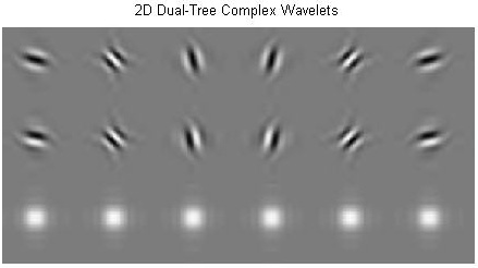
Note that the wavelets are oriented in the same six directions as those of the real 2-D dual-tree DWT. However, here we have two in each direction. If the six wavelets displayed on the first (second) row are interpreted as the real (imaginary) part of a set of six complex wavelets, then the magnitude of the six complex are shown on the third row. As shown in the figure, the magnitude of the complex wavelets do not have an oscillatory behavior - instead they are bell-shaped envelopes. This figure was produced with the following Matlab program (cplxdual2D_plots.m).

% cplxdual2D_plots
% DISPLAY 2D WAVELETS OF cplxdual2D.M

J = 4;
L = 3*2^(J+1);
N = L/2^J;
[Faf, Fsf] = FSfarras;
[af, sf] = dualfilt1;
x = zeros(2*L,6*L);
w = cplxdual2D(x, J, Faf, af);
w{J}{1}{2}{2}(N/2,N/2+0*N) = 1;
w{J}{1}{1}{3}(N/2,N/2+1*N) = 1;
w{J}{1}{2}{1}(N/2,N/2+2*N) = 1;
w{J}{1}{1}{1}(N/2,N/2+3*N) = 1;
w{J}{1}{2}{3}(N/2,N/2+4*N) = 1;
w{J}{1}{1}{2}(N/2,N/2+5*N) = 1;
w{J}{2}{2}{2}(N/2+N,N/2+0*N) = 1;
w{J}{2}{1}{3}(N/2+N,N/2+1*N) = 1;
w{J}{2}{2}{1}(N/2+N,N/2+2*N) = 1;
w{J}{2}{1}{1}(N/2+N,N/2+3*N) = 1;
w{J}{2}{2}{3}(N/2+N,N/2+4*N) = 1;
w{J}{2}{1}{2}(N/2+N,N/2+5*N) = 1;
y = icplxdual2D(w, J, Fsf, sf);
y = [y; sqrt(y(1:L,:).^2+y(L+[1:L],:).^2)];
figure(1)
clf
imagesc(y);
title('2D Dual-Tree Complex Wavelets')
axis image
axis off
colormap(gray(128))
print -djpeg95 cplxdual2D_plots

Summary of programs:

1. dualtree2D.m - Wavelet transform (real part)
2. idualtree2D.m - Inverse wavelet xform (real part)
3. dualtree2D_plots.m - Display wavelets (real part)
4. cplxdual2D.m - Complex wavelet xform
5. icplxdual2D.m - Inverse complex wavelet xform
6. cplxdual2D_plots.m - Display complex wavelets
7. pm.m - Plus and minus