TARA_Example2: Transient Artifact Reduction Algorithm (TARA)

TARA is designed to remove step and spike artifacts from data with low-frequency and white stochasitc components.

Contents

Start

clear
% close all

printme = @(filename) print('-dpdf', sprintf('figures/TARA_Example2_%s', filename));

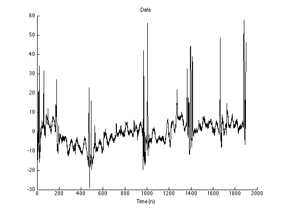
Load data

data = load('data/wl1_col02.txt');

y = data;

N = length(y);
n = 1:N;

figure(1)
clf
plot(y);
% xlim([900 1800])
box off
title('Data')
xlabel('Time (n)')

Set parameters

% Filter parameters:
fc = 0.03;          % fc : cut-off frequency (cycles/sample) (0 < fc < 0.5);
d = 1;              % d : filter order parameter (d = 1, 2, or 3)

% TARA parameters
theta = 0.05;
beta = 1.4;
ps = 1.0;   % psuedo sigma (psuedo noise)

Define filters

The high-pass filter is H = B*inv(A) where A and B are banded matrices (sparse data type in MATLAB)

[A, B, B1] = BAfilt(d, fc, N);

H = @(x) B*(A\x);           % H : high-pass filter

L = @(x) x - [nan(d,1); H(x); nan(d,1)];          % L : low-pass filter

x_lpf = L(y);               % x_lpf : Apply low-pass filter to data

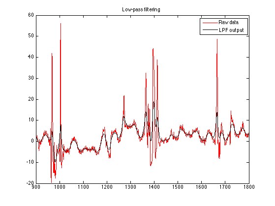
Low-pass filter (LPF)

Apply the low-pass filter to the data. Observe that the output of the low-pass filter does not closely follow the slowly varying background trend. The brief pulses in the data cause the output of the low-pass filter to deviate from the background trend.

figure(1)
clf
plot(n, y, 'r', n, x_lpf)
xlim([900 1800])
title('Low-pass filtering')
legend('Raw data', 'LPF output')

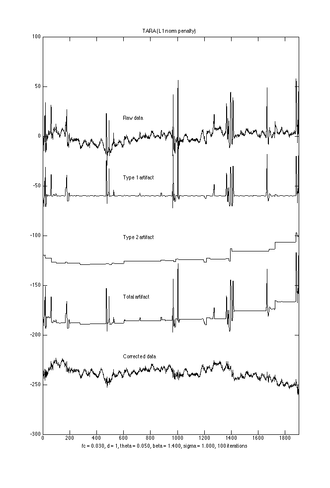
TARA with L1 norm penalty

TARA: Transient artifact reducation algortithm

Nit = 100;

% Run TARA
[x1, x2, f, cost, lam0, lam1, lam2] = tara2_L1(y, d, fc, theta, beta, ps, Nit);

txt = sprintf('fc = %.3f, d = %d, theta = %.3f, beta = %.3f, sigma = %.3f, %d iterations', fc, d, theta, beta, ps, Nit);

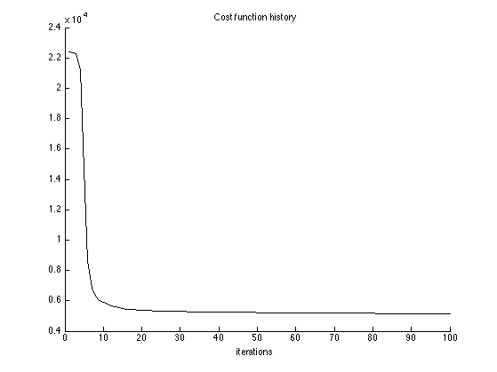
Cost function history

figure(1)
clf
plot(1:Nit, cost)
xlabel('iterations')
title('Cost function history')
box off

Display output

signals = [data x1 x2 x1+x2 data-x1-x2];
labels = {'Raw data','Type 1 artifact', 'Type 2 artifact', 'Total artifact', 'Corrected data'};
M = length(labels);
gap = 60;

figure(2)
clf
plot(n, bsxfun(@plus, -(0:M-1)*gap, signals), 'black')
% xlim([900 1800])
xlim([0 N])
tt = text(600*ones(1,M), gap*(0.3-(0:M-1)), labels);
title('TARA (L1 norm penalty)')
xlabel( txt )

orient tall
printme('L1')

Verifications

if 0
    % Verify that programs tara_L1 and tara2_L1 return the same output
    % signals:
    [x1_, x2_, f_, cost_] = tara_L1(y, d, fc, lam0, lam1, lam2, Nit);       % Run TARA

    % The following values should be zero or approximately zero
    disp( max(abs(x1 - x1_)) )
    disp( max(abs(x2 - x2_)) )
    disp( max(abs(f - f_)) )
    disp( max(abs(cost - cost_)) )
end

if 0
    % Verify that programs tara2 and tara2_L1 return the same output when pen = 'L1'
    pen = 'L1';
    [x1_, x2_, f_, cost_] = tara2(y, d, fc, theta, beta, ps, pen, 0, 0, 0, Nit);

    disp( max(abs(x1 - x1_)) )
    disp( max(abs(x2 - x2_)) )
    disp( max(abs(f - f_)) )
end

if 0
    % Verify that programs tara and tara2_L1 return the same output when pen = 'L1'
    pen = 'L1';
    [x1_, x2_, f_, cost_] = tara(y, d, fc, lam0, lam1, lam2, pen, 0, 0, 0, Nit);

    disp( max(abs(x1 - x1_)) )
    disp( max(abs(x2 - x2_)) )
    disp( max(abs(f - f_)) )
end

TARA with non-convex penalty

pen = 'atan';
r = 0.5;

% Initialize with L1 solution
[x1, x2, f, cost_, u1, u2] = tara2(y, d, fc, theta, beta, ps, 'L1', 0, 0, 0, Nit);
[x1_ncvx, x2_ncvx, f_ncvx, cost_ncvx] = tara2(y, d, fc, theta, beta, ps, pen, r, r, r, Nit, u1, u2);

txt2 = sprintf('%s penalty, r0 = %.2f, r1 = %.2f, r2 = %.2f', pen, r, r, r);

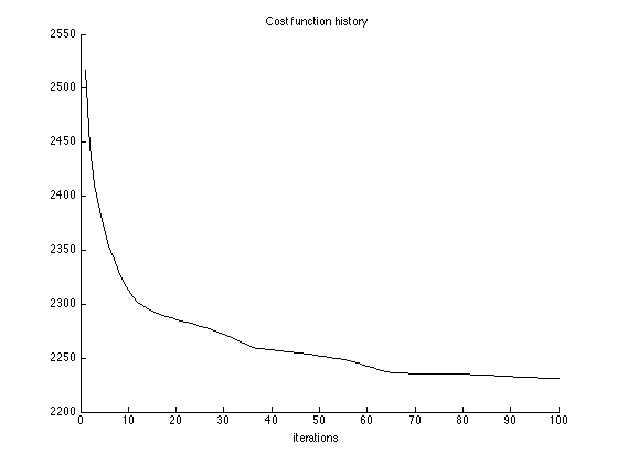
Cost function history

figure(1)
clf
plot(1:Nit, cost_ncvx)
xlabel('iterations')
title('Cost function history')
box off

Display output

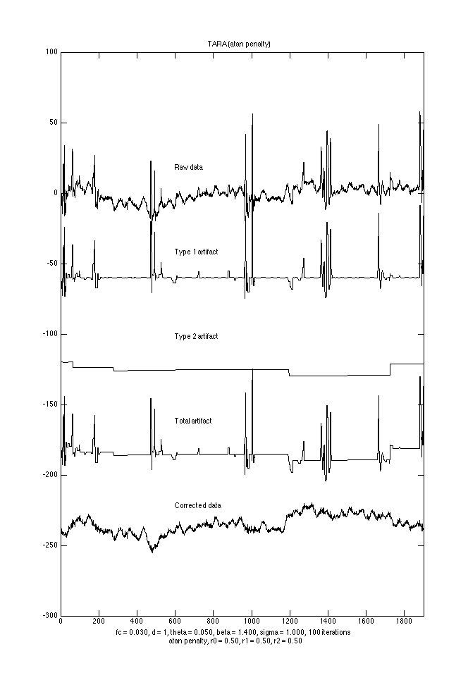
signals = [data x1_ncvx x2_ncvx x1_ncvx+x2_ncvx data-x1_ncvx-x2_ncvx];
labels = {'Raw data','Type 1 artifact', 'Type 2 artifact', 'Total artifact', 'Corrected data'};
M = length(labels);
gap = 60;

figure(2)
clf
plot(n, bsxfun(@plus, -(0:M-1)*gap, signals), 'black')
% xlim([900 1800])
xlim([0 N])
tt = text(600*ones(1,M), gap*(0.3-(0:M-1)), labels);
title('TARA (atan penalty)')
xlabel({txt, txt2})

orient tall
printme('atan')

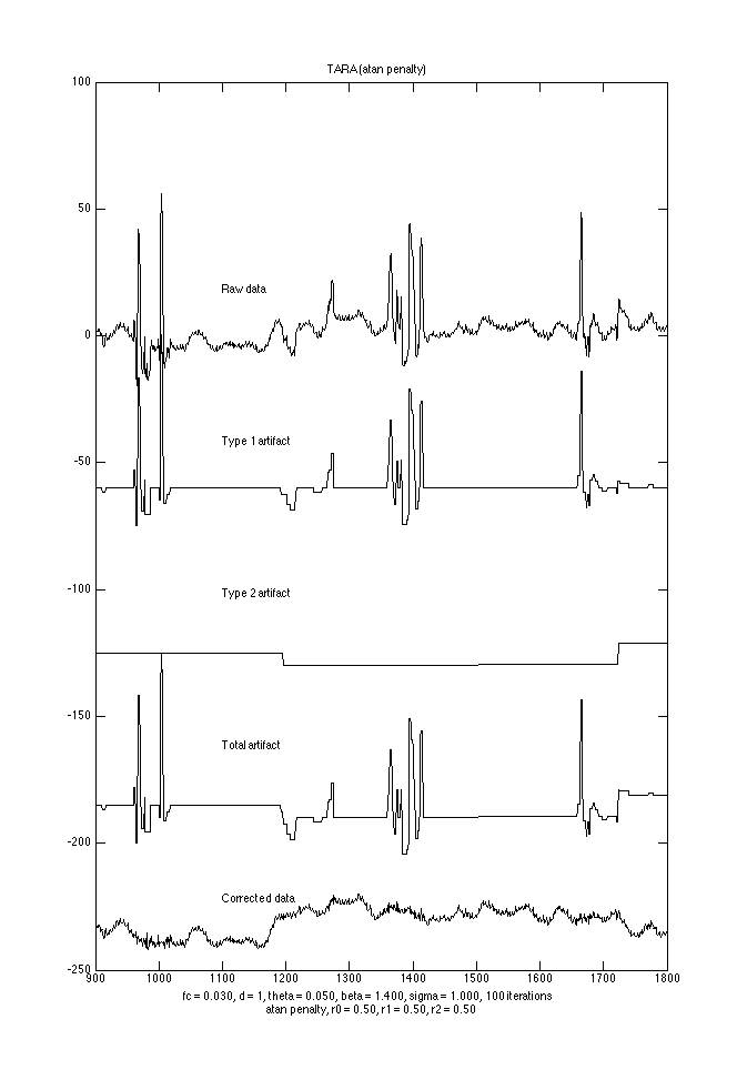
Display detail

xlim([900 1800])
tt = text(1100*ones(1,M), gap*(0.3-(0:M-1)), labels);

orient tall
printme('atan_detail')

Verification

if 0
    % Verify that 'tara' and 'tara2' return the same ouput
    [x1_ncvx, x2_ncvx, f_ncvx, cost_ncvx, u1, u2, lam0, lam1, lam2, a0, a1, a2] ...
        = tara2(y, d, fc, theta, beta, ps, pen, r, r, r, Nit, u1, u2);

    % Initialize with L1 solution
    [x1, x2, f, cost_, u1, u2] = tara(y, d, fc, lam0, lam1, lam2, 'L1', 0, 0, 0, Nit);
    [x1_ncvx_, x2_ncvx_, f_ncvx_, cost_ncvx_] = tara(y, d, fc, lam0, lam1, lam2, pen, a0, a1, a2, Nit, u1, u2);

    ma = @(x) max(abs(x(:)));
    disp( ma(x1_ncvx - x1_ncvx_) )
    disp( ma(x2_ncvx - x2_ncvx_) )
    disp( ma(f_ncvx - f_ncvx_) )
    disp( ma(cost_ncvx - cost_ncvx_) )

end

Published with MATLAB® 7.12