Frequency response demo

Illustration of the frequency response concept for discrete-time LTI systems.

Contents

Define system

The system is defined by the difference equation

y(n) = 0.2 x(n) - 0.3 x(n-1) + 0.2 x(n-2) + 1.8 y(n-1) - 0.9 * y(n-2)

clear

b = [0.2 -0.3  0.2];

a = [1 -1.8 0.9];

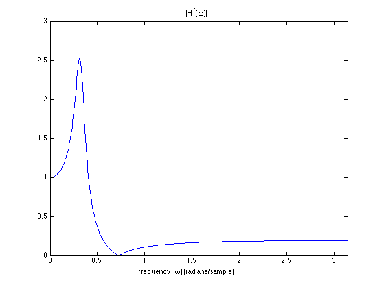
Plot frequency response (radians/sample)

Use the freqz function to calculate the frequency response.

[H, om] = freqz(b,a);       % om : frequency in units of radians/sample

figure(1)
clf
plot(om, abs(H))
title('|H^f(\omega)|')
xlabel('frequency (\omega) [radians/sample]')
xlim([0 pi])

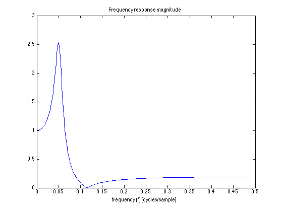
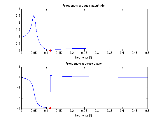
Use cycles/sample

Frequency axis in units of cycles/sample

f = om / (2*pi);            % f  : frequency in units of cycles/sample

figure(1)
clf
plot(f, abs(H))
title('Frequency response magnitude')
xlabel('frequency (f) [cycles/sample]')

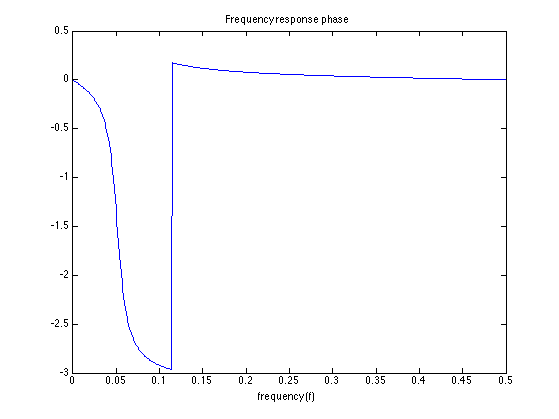
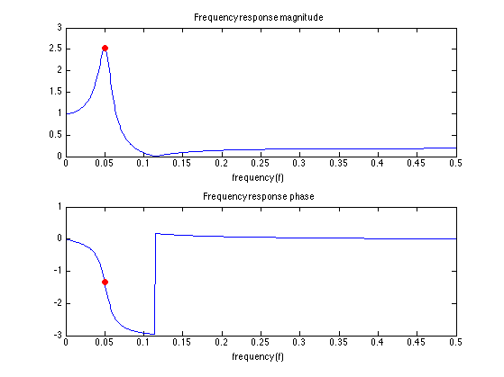
The phase response

Plot the phase of the frequency response. Why is there a discontinuity in the phase response? What is the size of the phase jump? At what frequency is the phase jump?

figure(1)
clf
plot(f, angle(H))
title('Frequency response phase')
xlabel('frequency (f)')

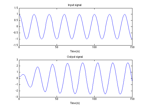
Define a cosine signal

om1 = 0.1*pi ;          % Frequency of cosine signal in units of radians/sample
f1 = om1/(2*pi);        % Cycles/sample

n = 0:150;
x = cos(om1*n);         % Input signal

Compute output signal

Use 'filter' to implement the difference equation.

y = filter(b, a, x);    % Output signal

figure(1)
clf
subplot(2, 1, 1)
plot(n, x)
title('Input signal')
xlabel('Time (n)')
ylim([-1.5 1.5])

subplot(2,1,2)
plot(n, y)
title('Output signal')
xlabel('Time (n)')

Use 'polyval' to evaluate the frequency response

Find the value of the frequency response at om1 by evaluating the transfer function at z1 = exp(j om1). Verify that the value agrees with 'freqz'.

I = sqrt(-1);
z1 = exp(I*om1);

H1 = polyval(b, z1) / polyval(a, z1);    % Value of frequency response at om1

abs(H1)
angle(H1)

ans =

    2.5381


ans =

   -1.3478

figure(1)
clf
subplot(2, 1, 1)
plot(f, abs(H), f1, abs(H1), 'ro', 'markerface', 'red')
title('Frequency response magnitude')
xlabel('frequency (f)')

subplot(2, 1, 2)
plot(f, angle(H), f1, angle(H1), 'ro', 'markerface', 'red')
title('Frequency response phase')
xlabel('frequency (f)')

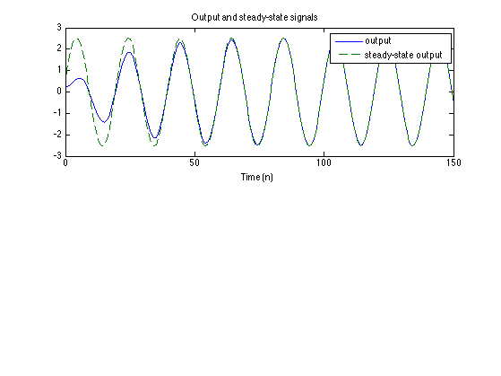
Formula for steady-state output

Use the value of the frequency response at om1 to compute the steady-state output signal. The output signal converges to the steady-state signal.

s = abs(H1) * cos(om1 * n + angle(H1));  % Steady-state output signal

figure(1)
clf
subplot(2, 1, 1)
plot(n, y, n, s, '--');
title('Output and steady-state signals')
xlabel('Time (n)')
legend('output', 'steady-state output')

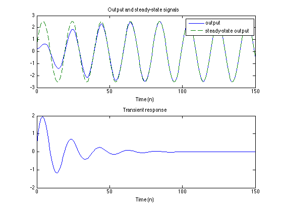
The transient response

We identify the transient response as the difference between the output signal and the steady-state output signal.

figure(1)
subplot(2, 1, 2)
plot(n, s-y);
title('Transient response')
xlabel('Time (n)')

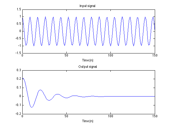
Compute output signal for another frequency

Create cosine signal with frequency om2 = 0.23*pi and compute the new output signal. Why does the output signal decay to zero? Can this be predicted directly from the frequency and/or the pole-zero diagram? [Hint: yes]

om2 = 0.23*pi;          % [radians/sample]
f2 = om2/(2*pi);        % [cycles/sample]
x = cos(om2*n);
y = filter(b, a, x);

figure(1)
clf
subplot(2,1,1)
plot(n, x)
title('Input signal')
xlabel('Time (n)')
ylim([-1.5 1.5])

subplot(2,1,2)
plot(n, y)
title('Output signal')
xlabel('Time (n)')

Pole-zero diagram

The nulls in the frequency response correspond to zeros on the unit circle.

figure(1)
clf
zplane(b, a)
title('Pole-zero diagram')

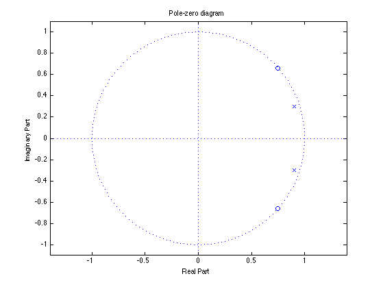
angle(roots(b))/pi

ans =

    0.2301
   -0.2301

Evaluate frequency response at second frequency.

Find frequency response value at om2. [Evaluate transfer function at z2 = exp(j om2)]. The value is almost zero. The value z2 is (almost) a zero of the transfer function.

z2 = exp(1j * om2);
H2 = polyval(b, z2) / polyval(a, z2);    % Value of frequency response at om2
abs(H2)

ans =

   1.1674e-04

figure(1)
clf
subplot(2, 1, 1)
plot(f, abs(H), f2, abs(H2), 'ro', 'markerface', 'red')
title('Frequency response magnitude')
xlabel('frequency (f)')

subplot(2, 1, 2)
plot(f, angle(H), f2, angle(H2), 'ro', 'markerface', 'red')
title('Frequency response phase')
xlabel('frequency (f)')

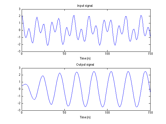
Two frequencies

The input consists of two cosine signal but the output signal consists of one cosine. The filter annilhates one of them. (Which one?)

x = 1.0 * cos(om1 * n) + 1.2 * cos(om2 * n);

y = filter(b, a, x);     % Output of filter

figure(1)
subplot(2, 1, 1)
plot(n, x)
title('Input signal')
xlabel('Time (n)')

subplot(2, 1, 2)
plot(n, y)
title('Output signal')
xlabel('Time (n)')

Published with MATLAB® 7.12