Examples of FIR filter design using Parks-McClellan algorithm

Use the Matlab function 'firpm'

Contents

Start

clear

Design FIR filter using Parks-McClellan algorithm

Low-pass filter design

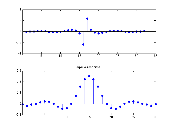
fp = 0.1;
fs = 0.15;

[h, del] = firpm(30, [0 fp fs .5]*2, [1 1 0 0]);

length(h)
del

figure(1)
stem(0:30, h, 'filled')
title('Impulse response')

ans =
    31
del =
    0.0241

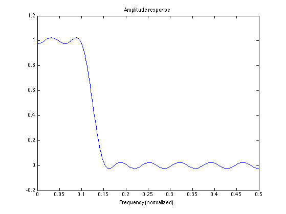
Compute amplitude response A

L = 512;
[A, om] = firamp(h, 1, L);

f = om/(2*pi);

figure(1)
clf
plot(f, A)
xlim([0 0.5])
title('Amplitude response')
xlabel('Frequency (normalized)')

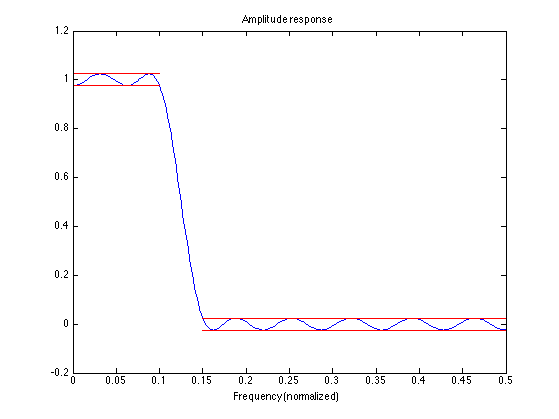
Plot with delta

figure(1)
clf
plot(f, A, [0 fp], (1-del)*[1 1],'r', [0 fp], (1+del)*[1 1], 'r', [fs 0.5], -del*[1 1], 'r', [fs 0.5], del*[1 1], 'r')
xlim([0 0.5])
title('Amplitude response')
xlabel('Frequency (normalized)')

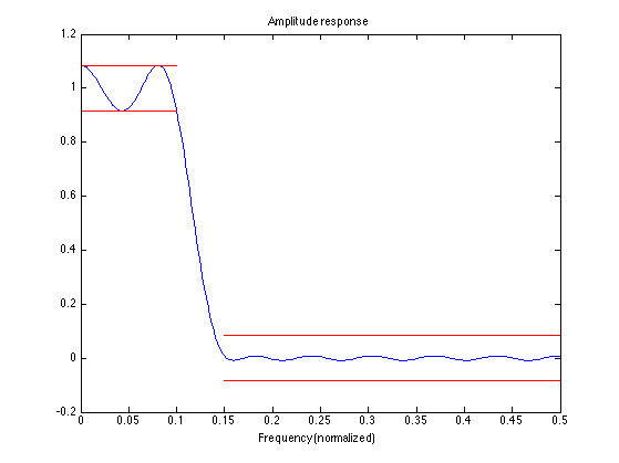
Use firpm with weighting

The weight function allows one to put more weight in one band than in the other band.

fp = 0.1;
fs = 0.15;

W = [1 10];

[h, del] = firpm(30, [0 fp fs .5]*2, [1 1 0 0], W);

del

del =
    0.0845

Compute amplitude response A

L = 512;
[A, om] = firamp(h, 1, L);

f = om/(2*pi);

% Oops. Pass-band and stop-band ripples are different in size
figure(1)
clf
plot(f, A, [0 fp], (1-del)*[1 1],'r', [0 fp], (1+del)*[1 1], 'r', [fs 0.5], -del*[1 1], 'r', [fs 0.5], del*[1 1], 'r')
xlim([0 0.5])
title('Amplitude response')
xlabel('Frequency (normalized)')

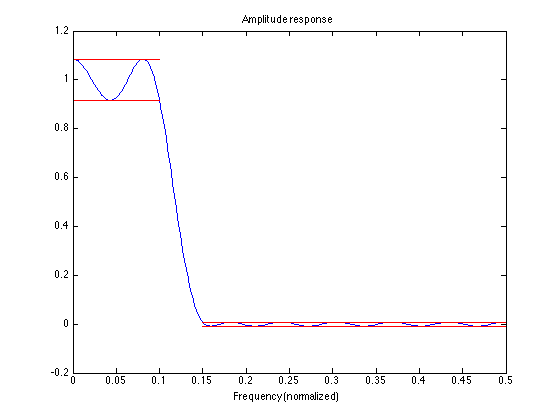
Plot with delta

Correct plot . . . Note: The stop-band ripple is one-tength the pass-band ripple

figure(1)
clf
plot(f, A, [0 fp], (1-del)*[1 1],'r', [0 fp], (1+del)*[1 1], 'r', [fs 0.5], -del/W(2)*[1 1], 'r', [fs 0.5], del/W(2)*[1 1], 'r')
xlim([0 0.5])
title('Amplitude response')
xlabel('Frequency (normalized)')

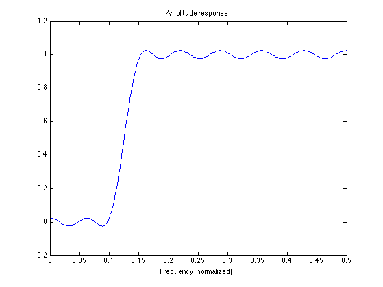
High-pass filter

fs = 0.1;
fp = 0.15;

[h, del] = firpm(30, [0 fs fp .5]*2, [0 0 1 1]);

L = 512;
[A, om] = firamp(h, 1, L);

figure(1)
clf
plot(f, A)
xlim([0 0.5])
title('Amplitude response')
xlabel('Frequency (normalized)')

High-pass filter (Even-length)

Why does this produce an error?

fs = 0.1;
fp = 0.15;

[h, del] = firpm(31, [0 fs fp .5]*2, [0 0 1 1]);

% Because 31 -> length(h) = 32 -> h is Type II -> Hf(pi) = 0
% which is inconsistent with the specification!

Warning: Odd order symmetric FIR filters must have a gain of zero
at the Nyquist frequency. The order is being increased by one.
Alternatively, you can pass a trailing 'h' argument,
as in firpm(N,F,A,W,'h'), to design a type 4 linear phase filter. 

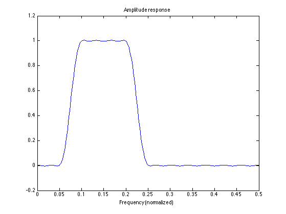
Band-pass filter

fs1 = 0.05;
fp1 = 0.1;
fp2 = 0.2;
fs2 = 0.25;

[h, del] = firpm(50, [0 fs1 fp1 fp2 fs2 .5]*2, [0 0 1 1 0 0]);

L = 512;
[A, om] = firamp(h, 1, L);

figure(1)
clf
plot(f, A)
xlim([0 0.5])
title('Amplitude response')
xlabel('Frequency (normalized)')

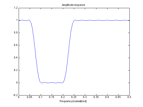
Band-stop filter

fp1 = 0.05;
fs1 = 0.1;
fs2 = 0.2;
fp2 = 0.25;

[h, del] = firpm(50, [0 fp1 fs1 fs2 fp2 .5]*2, [1 1 0 0 1 1]);

L = 512;
[A, om] = firamp(h, 1, L);

figure(1)
clf
plot(f, A)
xlim([0 0.5])
title('Amplitude response')
xlabel('Frequency (normalized)')

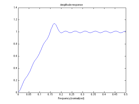
Custom filter

f1 = 0.15;
f2 = 0.2;

[h, del] = firpm(42, [0 f1 f2 .5]*2, [0 1 1 1]);

L = 512;
A = firamp(h, 1, L);

figure(1)
clf
plot(f, A)
xlim([0 0.5])
title('Amplitude response')
xlabel('Frequency (normalized)')

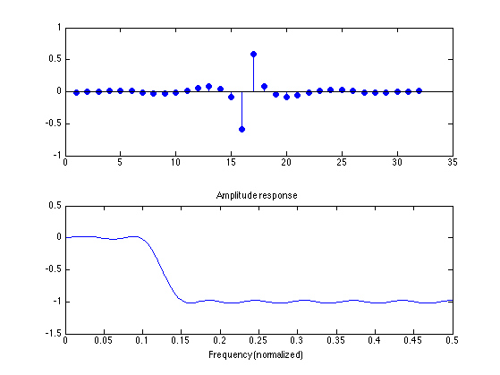
Type III and Type IV FIR filters

To obtain an anti-symmetric impulse response, use 'hilbert' in firpm. In this case, we must have Hf(0) = 0.

fs = 0.1;
fp = 0.15;

[h, del] = firpm(31, [0 fs fp .5]*2, [0 0 1 1], 'hilbert');

L = 512;
A = firamp(h, 3, L);

figure(1)
clf
subplot(2, 1, 1)
stem(h, 'filled')
subplot(2, 1, 2)
plot(f, A)
xlim([0 0.5])
title('Amplitude response')
xlabel('Frequency (normalized)')

Published with MATLAB® 7.12