Filter delay demo
Illustratation of delay induced by an LTI system.
Contents
Start
clear
% close all
Define system
The system is defined by the difference equation
y(n) = 0.1 x(n) - 0.1 x(n-1) + 0.1 x(n-2) + 1.5 y(n-1) - 0.8 * y(n-2)
b = 0.1*[1 -1  1];

a = [1 -1.5 0.8];
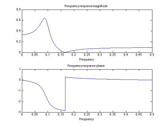
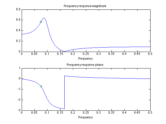
Plot frequency response
Use the 'freqz' function to calculate the frequency response.
[H, om] = freqz(b,a);
f = om / (2*pi);

figure(1)
clf

subplot(2, 1, 1)
plot(f, abs(H))
title('Frequency response magnitude')
xlabel('Frequency')

subplot(2, 1, 2)
plot(f, angle(H))
title('Frequency response phase')
xlabel('Frequency')
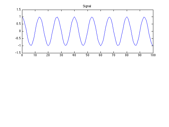
Create sinusoid
Create a sinusoid with a specified frequency
L = 100;
n = 0:L;

om1 = 0.15*pi;      % Frequency of sinusoid radians/sample
f1 = om1 / (2*pi);  % Frequency in cycles/sample

x = cos(om1*n);     % Cosine signal

figure(1)
clf
subplot(2,1,1)
plot(n, x)
title('Signal')
ylim([-1.5 1.5])
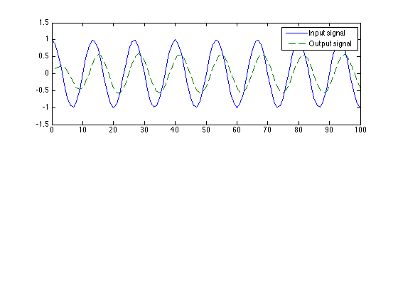
Output signal
Comput output signal. Plot input and output signals on the same plot. Notice the output signal is delayed with respect to the input signal. How many samples is the input signal delayed?
y = filter(b, a, x);    % Output signal

figure(1)
clf
subplot(2, 1, 1)
plot(n, x, n, y, '--')
legend('Input signal', 'Output signal')
ylim([-1.5 1.5])
Frequency response value at om1
The value H(om1) of the frequency response at om1 is a complex number.
I = sqrt(-1);
z1 = exp(I*om1);
d = length(b) - length(a);
H_om1 = 1/z1^d * polyval(b, z1) / polyval(a, z1)    % Value of frequency response at om1
H_om1 =

   0.4268 - 0.3733i
Magnitude at om1
H(om1)
A = abs(H_om1)
A =

    0.5670
Phase at om1
The angle of H(om1) will tell us the delay..
theta = angle(H_om1)
theta =

   -0.7186
Show magnitude and phase on frequency response plot
figure(1)
clf

subplot(2, 1, 1)
plot(f, abs(H), f1, A, 'o')
title('Frequency response magnitude')
xlabel('Frequency')

subplot(2, 1, 2)
plot(f, angle(H), f1, theta, 'o')
title('Frequency response phase')
xlabel('Frequency')
Delay (in samples) at om1
Compute the signal delay in samples
M = -angle(H_om1)/om1      % Delay in samples

fprintf('The delay is %.2f samples\n', M)
M =

    1.5250

The delay is 1.52 samples
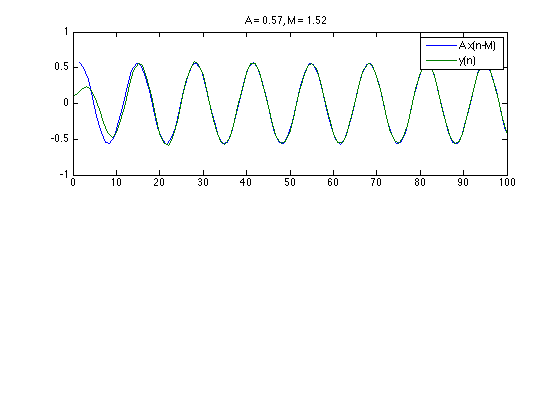
Verify delay property
Plot the input and output signal together, where the input signal is delayed by M samples and multiplied by A. Observed that the output signal y(n) is in phase with the delayed input signal A x(n-M).
figure(1)
clf
subplot(2, 1, 1)
plot(n + M, A*x, n, y)
xlim([0 L])
legend('A x(n-M)', 'y(n)')
title( sprintf('A = %.2f, M = %.2f', A, M) )
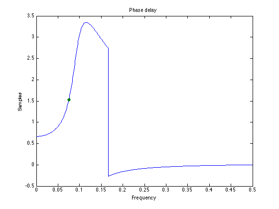
Plot phase delay function
Show delay M on plot of phase delay function.
figure(1)
clf
plot(f, -angle( H )./om, f1, M, '.', 'markersize', 20)
title('Phase delay')
ylabel('Samples')
xlabel('Frequency')