Matlab demo - filter

In class Matlab demo EE 3054 September 22, 2014

Contents

help filter

 FILTER One-dimensional digital filter.
    Y = FILTER(B,A,X) filters the data in vector X with the
    filter described by vectors A and B to create the filtered
    data Y.  The filter is a "Direct Form II Transposed"
    implementation of the standard difference equation:
 
    a(1)*y(n) = b(1)*x(n) + b(2)*x(n-1) + ... + b(nb+1)*x(n-nb)
                          - a(2)*y(n-1) - ... - a(na+1)*y(n-na)
 
    If a(1) is not equal to 1, FILTER normalizes the filter
    coefficients by a(1). 
 
    FILTER always operates along the first non-singleton dimension,
    namely dimension 1 for column vectors and non-trivial matrices,
    and dimension 2 for row vectors.
 
    [Y,Zf] = FILTER(B,A,X,Zi) gives access to initial and final
    conditions, Zi and Zf, of the delays.  Zi is a vector of length
    MAX(LENGTH(A),LENGTH(B))-1, or an array with the leading dimension 
    of size MAX(LENGTH(A),LENGTH(B))-1 and with remaining dimensions 
    matching those of X.
 
    FILTER(B,A,X,[],DIM) or FILTER(B,A,X,Zi,DIM) operates along the
    dimension DIM.
 
    See also FILTER2, FILTFILT, FILTIC.
 
    Note: FILTFILT and FILTIC are in the Signal Processing Toolbox.

    Overloaded methods:
       SigLogSelector.filter
       gf/filter
       channel.filter
       gpuArray/filter
       gjr/filter
       garch/filter
       egarch/filter
       arima/filter
       LagOp/filter
       mfilt.filter
       adaptfilt.filter
       fints/filter
       fxptui.filter
       dfilt.filter
       timeseries/filter

    Reference page in Help browser
       doc filter

Difference equation

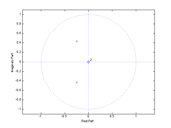
y(n) = x(n) - (1/2) y(n-1) - (1/4) y(n-2)

b = 1;
a = [1 1/2 1/4]
roots(a)

% We found the poles were 0.5 * exp(+/- 2*pi/3 * i)

0.5 * exp(2*pi/3 * i)   % agrees with 'roots'

a =

    1.0000    0.5000    0.2500


ans =

  -0.2500 + 0.4330i
  -0.2500 - 0.4330i


ans =

  -0.2500 + 0.4330i

Pole/zero diagram

zplane(b, a)

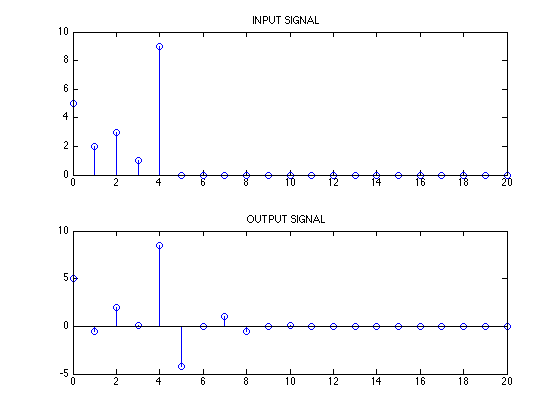
Run difference equation

% Make input signal
x = zeros(1, 21);
x(1:5) = [5 2 3 1 9];

n = 0:20;

% plot input signal x
subplot(2, 1, 1)
stem(n, x)
title('INPUT SIGNAL')

% compute output signal y
y = filter(b, a, x);

% plot output signal y
subplot(2, 1, 2)
stem(n, y)
title('OUTPUT SIGNAL')

Find impulse response

imp = [1 zeros(1, 20)];
h = filter(b, a, imp);

figure(2)
subplot(2, 1, 1)
stem(n, imp)
title('IMPULSE')
subplot(2, 1, 2)
stem(n, h)
title('IMPULSE RESPONSE')

% adjust plot axes
for k = 1:2
    subplot(2, 1, k)
    xlim([-2 20])
    ylim([-1 2])
end

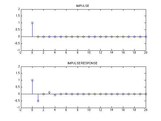
Verify formula

% Our formula for the impulse response:
h2 = 2/sqrt(3) * (1/2).^n .* cos(2*pi/3 * n + pi/6);

[h' h2' (h-h2)']
% impulse response formula is same as impulse response numerically computed using 'filter' function

ans =

    1.0000    1.0000   -0.0000
   -0.5000   -0.5000         0
         0   -0.0000    0.0000
    0.1250    0.1250         0
   -0.0625   -0.0625   -0.0000
         0   -0.0000    0.0000
    0.0156    0.0156   -0.0000
   -0.0078   -0.0078   -0.0000
         0   -0.0000    0.0000
    0.0020    0.0020   -0.0000
   -0.0010   -0.0010   -0.0000
         0   -0.0000    0.0000
    0.0002    0.0002   -0.0000
   -0.0001   -0.0001   -0.0000
         0   -0.0000    0.0000
    0.0000    0.0000   -0.0000
   -0.0000   -0.0000   -0.0000
         0   -0.0000    0.0000
    0.0000    0.0000    0.0000
   -0.0000   -0.0000   -0.0000
         0   -0.0000    0.0000

Published with MATLAB® R2013a